SETUP

library( foreign )
library( memisc )
library( knitr )
library( dplyr )
library( xtable )
library( stargazer )
library( broom )
library( pander )

LOAD DATA

dat <- readRDS( "./Data/CompleteHazardSpells.rds" )

# lapply( dat, class )
#                   
# head( dat, 25 ) %>% pander

nrow( dat )

## [1] 22026

MODEL WITH CONTINUOUS AGE

Continuous Duration

m.01.01 <- glm( formula= prof ~ AGE, data=dat,  family=binomial("logit") )
m.01.02 <- glm( formula= prof ~ AGE + Age2, data=dat,  family=binomial("logit") )
m.01.03 <- glm( formula= prof ~ AGE + Age2 + Age3, data=dat,  family=binomial("logit") )
m.01.04 <- glm( formula= prof ~ AGE + Age2 + Age3 + Age4 + Age5, data=dat,  family=binomial("logit") )


m.01.01 %>% tidy %>% kable( digits=3 )

term	estimate	std.error	statistic	p.value
(Intercept)	-2.351	0.052	-45.174	0
AGE	0.079	0.013	5.955	0

m.01.02 %>% tidy %>% kable( digits=3 )

term	estimate	std.error	statistic
(Intercept)	-4.449	0.134	-33.083
AGE	1.483	0.079	18.861
Age2	-0.195	0.011	-18.329

m.01.03 %>% tidy %>% kable( digits=3 )

term	estimate	std.error	statistic
(Intercept)	-9.657	0.409	-23.636
AGE	6.820	0.372	18.325
Age2	-1.801	0.105	-17.112
Age3	0.146	0.009	15.765

m.01.04 %>% tidy %>% kable( digits=3 )

term	estimate	std.error	statistic	p.value
(Intercept)	-98.285	716.190	-0.137	0.891
AGE	137.309	1038.478	0.132	0.895
Age2	-74.921	576.934	-0.130	0.897
Age3	19.722	154.181	0.128	0.898
Age4	-2.516	19.894	-0.126	0.899
Age5	0.125	0.995	0.125	0.900

par( mfrow=c(2,2) )

plot( dat$AGE , m.01.01$fitted.values, pch=19, cex=2, bty="n" )
plot( dat$AGE , m.01.02$fitted.values, pch=19, cex=2, bty="n" )
plot( dat$AGE , m.01.03$fitted.values, pch=19, cex=2, bty="n" )
plot( dat$AGE , m.01.04$fitted.values, pch=19, cex=2, bty="n" )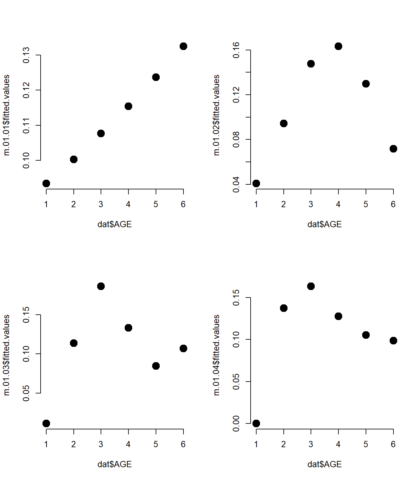

DISCRETE TIME MODEL

Discrete Duration

m.02 <- glm( formula= prof ~ D1 + D2 + D3 + D4 + D5 + D6 - 1, data=dat,   family=binomial("logit") )

m.02 %>% tidy %>% kable( digits=3 )

term	estimate	std.error	statistic	p.value
D1	-18.566	119.365	-0.156	0.876
D2	-1.839	0.043	-42.385	0.000
D3	-1.634	0.042	-39.027	0.000
D4	-1.922	0.048	-40.104	0.000
D5	-2.139	0.056	-37.966	0.000
D6	-2.213	0.060	-36.867	0.000

# stargazer( m.02, type = 'html')

pd <- unique( data.frame( age=dat$age, hazard.rate=m.02$fitted.values ) )

pd <- pd[ order(pd$age) , ]

plot( pd$age, pd$hazard.rate, type="b", pch=19, col="gray20", cex=2, xlab="NP Age", ylab="Hazard Rate" )

# points( (dat$AGE - 1) , m.01$fitted.values, pch=19, cex=2, col="red" )

    



m.03 <- glm( formula= prof ~ D1 + D2 + D3 + D4 + D5 + D6 + Accrual + GovtMoneyRat + HHI + 
                             UNAgrand + FixedCostRat + SurplusRat_ndrop_w892 + EqRat_w_K + 
                             ProfFundFeeYes - 1, 
                             data=dat,   family=binomial("logit") )

m.03 %>% tidy %>% kable( digits=3 )

term	estimate	std.error	statistic	p.value
D1	-19.205	174.151	-0.110	0.912
D2	-1.391	0.107	-13.039	0.000
D3	-1.162	0.104	-11.147	0.000
D4	-1.390	0.107	-13.015	0.000
D5	-1.562	0.112	-14.007	0.000
D6	-1.617	0.114	-14.242	0.000
Accrual	0.611	0.054	11.254	0.000
GovtMoneyRat	1.269	0.096	13.169	0.000
HHI	-0.526	0.111	-4.751	0.000
UNAgrand	0.001	0.000	5.573	0.000
FixedCostRat	0.247	0.173	1.428	0.153
SurplusRat_ndrop_w892	1.904	0.083	22.879	0.000
EqRat_w_K	0.001	0.000	5.071	0.000
ProfFundFeeYes	1.065	0.110	9.708	0.000

Survival Curves

This is the intercept only model, not accounting for any covariates (not very good model).

# Control case - no professionalization

h1 <- (    1 / ( 1 + exp(-( m.03$coeff[1] ))   )     )
h2 <- (    1 / ( 1 + exp(-( m.03$coeff[2] ))   )     )
h3 <- (    1 / ( 1 + exp(-( m.03$coeff[3] ))   )     )
h4 <- (    1 / ( 1 + exp(-( m.03$coeff[4] ))   )     )
h5 <- (    1 / ( 1 + exp(-( m.03$coeff[5] ))   )     )
h6 <- (    1 / ( 1 + exp(-( m.03$coeff[6] ))   )     )

hr <- data.frame( age=0:5, hazard.rate=c(h1,h2,h3,h4,h5,h6) ) 

sr <- cumprod( (1-hr$hazard.rate))

hr <- cbind( hr, survival.rate=sr )

hr

par( mfrow=c(1,2) )

plot( 0:5, hr$hazard.rate, type="b", pch=19, cex=1.2, ylim=c(0,0.5),
      main="Hazard Rate", xlab="Nonprofit Age", ylab="Probability of Professionalizing at Age=j")

plot( 0:5, sr, type="b", pch=19, cex=1.2, ylim=c(0,1.1),
      main="Survival Curve", xlab="Nonprofit Age", ylab="Probability of Remaining Nonprofessional")
abline( h=0.5, col="red", lty=3)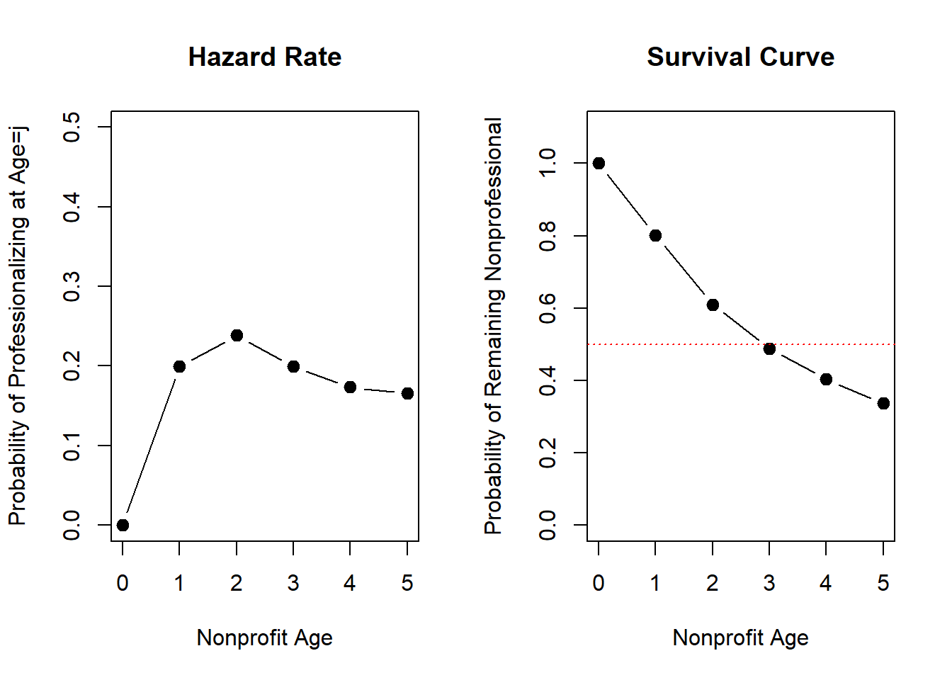

Centered Estimates

Hold each

# m.03 <- glm( formula= prof ~ D1 + D2 + D3 + D4 + D5 + D6 + Accrual + GovtMoneyRat + HHI + UNAgrand + 
#                              FixedCostRat + SurplusRat_ndrop_w892 + EqRat_w_K + ProfFundFeeYes - 1, 
#                              data=dat,   family=binomial("logit") )


coef.names <- c("D1","D2","D3","D4","D5","D6","Accrual","GovtMoneyRat", 
                 "HHI","UNAgrand","FixedCostRat","SurplusRat_ndrop_w892", 
                 "EqRat_w_K","ProfFundFeeYes" )

# only IVs in the model

td <- dat[ , c("Accrual","GovtMoneyRat","HHI","UNAgrand","FixedCostRat","SurplusRat_ndrop_w892","EqRat_w_K","ProfFundFeeYes") ]


period1 <- c( c(1,0,0,0,0,0), unlist( lapply( td, quantile, 0.50, na.rm=T ) ) )
period2 <- c( c(0,1,0,0,0,0), unlist( lapply( td, quantile, 0.50, na.rm=T ) ) )
period3 <- c( c(0,0,1,0,0,0), unlist( lapply( td, quantile, 0.50, na.rm=T ) ) )
period4 <- c( c(0,0,0,1,0,0), unlist( lapply( td, quantile, 0.50, na.rm=T ) ) )
period5 <- c( c(0,0,0,0,1,0), unlist( lapply( td, quantile, 0.50, na.rm=T ) ) )
period6 <- c( c(0,0,0,0,0,1), unlist( lapply( td, quantile, 0.50, na.rm=T ) ) )

# period1[12] <- median(dat$SurplusRat_ndrop_w892, na.rm=T)

# period1 <- c(1,0,0,0,0,0, 0,0,0.54,0,0,-0.49853,1.9,0)
# period2 <- c(0,1,0,0,0,0, 0,0,0.54,0,0,-0.49853,1.9,0)
# period3 <- c(0,0,1,0,0,0, 0,0,0.54,0,0,-0.49853,1.9,0)
# period4 <- c(0,0,0,1,0,0, 0,0,0.54,0,0,-0.49853,1.9,0)
# period5 <- c(0,0,0,0,1,0, 0,0,0.54,0,0,-0.49853,1.9,0)
# period6 <- c(0,0,0,0,0,1, 0,0,0.54,0,0,-0.49853,1.9,0)


h1 <- (    1 / ( 1 + exp(-( sum(period1 * m.03$coefficients) ))   )     )
h2 <- (    1 / ( 1 + exp(-( sum(period2 * m.03$coefficients) ))   )     )
h3 <- (    1 / ( 1 + exp(-( sum(period3 * m.03$coefficients) ))   )     )
h4 <- (    1 / ( 1 + exp(-( sum(period4 * m.03$coefficients) ))   )     )
h5 <- (    1 / ( 1 + exp(-( sum(period5 * m.03$coefficients) ))   )     )
h6 <- (    1 / ( 1 + exp(-( sum(period6 * m.03$coefficients) ))   )     )

hrc <- data.frame( age=1:6, hazard.rate=round(c(h1,h2,h3,h4,h5,h6),4) ) 

src <- cumprod( (1-hrc$hazard.rate))

hrc <- cbind( hrc, survival.rate=src )

hrc

par( mfrow=c(1,2) )

plot( 1:6, hrc$hazard.rate, type="b", pch=19, cex=1.2, bty="n",
      main="Hazard Rate", xlab="Nonprofit Age", ylab="Probability of Professionalizing at Age=j")

plot( 1:6, src, type="b", pch=19, cex=1.2, ylim=c(0,1.1), bty="n",
      main="Survival Curve", xlab="Nonprofit Age", ylab="Probability of Remaining Nonprofessional")
abline( h=0.5, col="red", lty=3)

FULL MODELS

###  ALL

m.all <- glm( formula= prof ~ D1 + D2 + D3 + D4 + D5 + D6 + Accrual + GovtMoneyRat + HHI + 
                             UNAgrand + FixedCostRat + SurplusRat_ndrop_w892 + EqRat_w_K + 
                             ProfFundFeeYes - 1, 
                             data=dat,   family=binomial("logit") )
                             

############## HEALTH

dat.health <- dat[ dat$Subsector2 == "Health", ]

m.health <- glm( formula= prof ~ D1 + D2 + D3 + D4 + D5 + D6 + Accrual + GovtMoneyRat + HHI + 
                             UNAgrand + FixedCostRat + SurplusRat_ndrop_w892 + EqRat_w_K + 
                             ProfFundFeeYes - 1, 
                             data=dat.health,   family=binomial("logit") )

# summary( m.04 )




############ HUMAN SERVICES

dat.hs <- dat[ dat$Subsector2 == "Human Svcs", ]

m.hs <- glm( formula= prof ~ D1 + D2 + D3 + D4 + D5 + D6 + Accrual + GovtMoneyRat + HHI + 
                             UNAgrand + FixedCostRat + SurplusRat_ndrop_w892 + EqRat_w_K + 
                             ProfFundFeeYes - 1, 
                             data=dat.hs,   family=binomial("logit") )

# summary( m.05 )


############ ARTS

dat.arts <- dat[ dat$Subsector2 == "Arts", ]

m.arts <- glm( formula= prof ~ D1 + D2 + D3 + D4 + D5 + D6 + Accrual + GovtMoneyRat + HHI + 
                             UNAgrand + FixedCostRat + SurplusRat_ndrop_w892 + EqRat_w_K + 
                             ProfFundFeeYes - 1, 
                             data=dat.arts,   family=binomial("logit") )

# summary( m.06 )


############# EDUCATION

dat.edu <- dat[ dat$Subsector2 == "Edu(Exclu Higher)" , ]

m.edu <- glm( formula= prof ~ D1 + D2 + D3 + D4 + D5 + D6 + Accrual + GovtMoneyRat + HHI + 
                             UNAgrand + FixedCostRat + SurplusRat_ndrop_w892 + EqRat_w_K + 
                             ProfFundFeeYes - 1, 
                             data=dat.edu,   family=binomial("logit") )

# summary( m.07 )


# ############# HIGHER ED AND HOSPITALS
# 
# dat.hos <- dat[ dat$Subsector2 == "Higher Edu or Hospitals" , ]
# 
# m.08 <- glm( formula= prof ~ D1 + D2 + D3 + D4 + D5 + D6 + Accrual + GovtMoneyRat + HHI + 
#                              UNAgrand + FixedCostRat + SurplusRat_ndrop_w892 + EqRat_w_K + 
#                              ProfFundFeeYes - 1, 
#                              data=dat.hos,   family=binomial("logit") )
# 
# # summary( m.08 )



############# PUBLIC

dat.pub <- dat[ dat$Subsector2 == "Public" , ]

m.pub <- glm( formula= prof ~ D1 + D2 + D3 + D4 + D5 + D6 + Accrual + GovtMoneyRat + HHI + 
                             UNAgrand + FixedCostRat + SurplusRat_ndrop_w892 + EqRat_w_K + 
                             ProfFundFeeYes - 1, 
                             data=dat.pub,   family=binomial("logit") )

# summary( m.09 )


############# OTHER

dat.other <- dat[ dat$Subsector2 == "Other"  , ]

m.other <- glm( formula= prof ~ D1 + D2 + D3 + D4 + D5 + D6 + Accrual + GovtMoneyRat + HHI + 
                             UNAgrand + FixedCostRat + SurplusRat_ndrop_w892 + EqRat_w_K + 
                             ProfFundFeeYes - 1, 
                             data=dat.other,   family=binomial("logit") )

# summary( m.10 )



# mtable123 <- mtable( "Combined"=m.03, "Arts"=m.06, "Health"=m.04,
#                      "Human Services"=m.05, "Public"=m.09, "Education"=m.07, 
#                      "Misc."=m.10,
#                      summary.stats=c("p","N") )
# 
# 
# panderOptions("digits", 2)
# 
# mtable123 # %>% pander

Output

# stargazer(linear.1, linear.2, probit.model, title="Regression Results",
# align=TRUE, dep.var.labels=c("Overall Rating","High Rating"),
# covariate.labels=c("Handling of Complaints","No Special Privileges",
# "Opportunity to Learn","Performance-Based Raises","Too Critical","Advancement"),
# omit.stat=c("LL","ser","f"), no.space=TRUE)


stargazer( m.all, m.arts, m.health, m.hs, m.pub, m.edu, m.other, type="html", digits=2,
           column.labels=c("All","Arts","Health","Human Services","Public","Education","Misc"),
           title="Discrete Hazard Model Estimates",
           dep.var.labels=c("Professionalization"),
           no.space = TRUE,
           out="./Results/RegTables.doc"
         )

**Discrete Hazard Model Estimates**

	Dependent variable:

	Professionalization
	All	Arts	Health	Human Services	Public	Education	Misc
	(1)	(2)	(3)	(4)	(5)	(6)	(7)

D1	-19.20	-19.16	-19.70	-17.98	-25.38	-18.80	-19.19
	(174.15)	(513.52)	(615.08)	(176.70)	(451.84)	(424.06)	(407.63)
D2	-1.39^***	-1.79^***	-2.06^***	-1.26^***	-1.31^***	-1.09^***	-1.58^***
	(0.11)	(0.33)	(0.45)	(0.17)	(0.33)	(0.28)	(0.30)
D3	-1.16^***	-1.37^***	-1.61^***	-1.08^***	-1.12^***	-0.83^***	-1.46^***
	(0.10)	(0.33)	(0.42)	(0.16)	(0.32)	(0.28)	(0.29)
D4	-1.39^***	-1.65^***	-1.73^***	-1.23^***	-1.41^***	-1.12^***	-1.75^***
	(0.11)	(0.32)	(0.43)	(0.17)	(0.32)	(0.28)	(0.30)
D5	-1.56^***	-1.76^***	-2.28^***	-1.45^***	-1.25^***	-1.37^***	-1.82^***
	(0.11)	(0.33)	(0.46)	(0.18)	(0.33)	(0.30)	(0.31)
D6	-1.62^***	-1.64^***	-2.26^***	-1.54^***	-1.73^***	-1.22^***	-1.82^***
	(0.11)	(0.33)	(0.48)	(0.18)	(0.35)	(0.30)	(0.32)
Accrual	0.61^***	0.78^***	0.81^***	0.54^***	0.46^***	0.81^***	0.46^***
	(0.05)	(0.17)	(0.19)	(0.09)	(0.15)	(0.14)	(0.16)
GovtMoneyRat	1.27^***	1.26^***	0.93^***	1.07^***	1.87^***	1.69^***	1.39^***
	(0.10)	(0.45)	(0.34)	(0.13)	(0.25)	(0.34)	(0.32)
HHI	-0.53^***	-0.51	0.42	-0.63^***	-0.72^**	-1.26^***	0.29
	(0.11)	(0.34)	(0.43)	(0.18)	(0.34)	(0.30)	(0.31)
UNAgrand	0.001^***	0.002^**	0.002^*	0.0004^**	0.002^***	0.001^*	0.005^***
	(0.0002)	(0.001)	(0.001)	(0.0002)	(0.0005)	(0.001)	(0.001)
FixedCostRat	0.25	0.24	-0.47	0.48^**	-0.56	1.46^**	-0.93^*
	(0.17)	(0.65)	(0.67)	(0.24)	(0.65)	(0.61)	(0.50)
SurplusRat_ndrop_w892	1.90^***	2.53^***	1.41^***	1.96^***	1.62^***	1.93^***	1.75^***
	(0.08)	(0.28)	(0.26)	(0.14)	(0.21)	(0.23)	(0.21)
EqRat_w_K	0.001^***	0.001^**	-0.0003	0.001^***	0.002^***	0.001	-0.001
	(0.0002)	(0.001)	(0.001)	(0.0004)	(0.0005)	(0.001)	(0.001)
ProfFundFeeYes	1.06^***	1.32^***	1.09^***	0.95^***	1.36^***	1.51^***	0.57^*
	(0.11)	(0.32)	(0.36)	(0.17)	(0.36)	(0.31)	(0.31)

Observations	22,026	2,512	1,402	7,696	2,839	3,745	3,832
Log Likelihood	-5,470.23	-567.86	-389.40	-2,049.47	-691.98	-914.79	-776.28
Akaike Inf. Crit.	10,968.47	1,163.72	806.80	4,126.94	1,411.97	1,857.59	1,580.57

Note:	p<0.1; p<0.05; p<0.01

Specification

Jesse Lecy

SETUP

LOAD DATA

MODEL WITH CONTINUOUS AGE

Continuous Duration

DISCRETE TIME MODEL

Discrete Duration

Survival Curves

Centered Estimates

FULL MODELS

Output