Part 1 — Regression Foundations
Builds a bivariate regression model from the ground up: sample variance, the slope and intercept, residuals, and the decomposition of the total sum of squares. The running example asks whether caffeine raises heart rate, a question that is easy to model and hard to interpret.
Reference material
-
Using Regression Models to Estimate Program Effects
Reichardt, C. S., & Bormann, C. A. (1994). Handbook of Practical Program Evaluation.
-
Applied Regression: An Introduction
Lewis-Beck, C., & Lewis-Beck, M. (2015). Sage. Reference for the core formulas.
-
OpenIntro Statistics, Ch. 8 — Introduction to Linear Regression
Diez, D. M., Barr, C. D., & Cetinkaya-Rundel, M. (2012).
-
Regression Review Self-Test
Benchmark your baseline knowledge before starting the sequence.
-
Common Statistics Notation
One-page key to the symbols used throughout the lectures.
Traces a confidence interval back to its parts, from standard errors to the residuals and model they are built from. The key distinction is between the spread of the data (standard deviation) and the spread of estimates across repeated samples (standard error).
Moves from bivariate to multiple regression and shows the two different things a control variable can do. Controls related only to the outcome shrink standard errors, while controls related to both the treatment and the outcome change the slope.
A variable left out of a model does not disappear; its effect is absorbed into the slopes of the variables that remain, by an amount you can calculate. The crack-baby research and the doctor-patient racial concordance debate show how omitted variables produce confident but wrong conclusions, and why randomization breaks the bias.
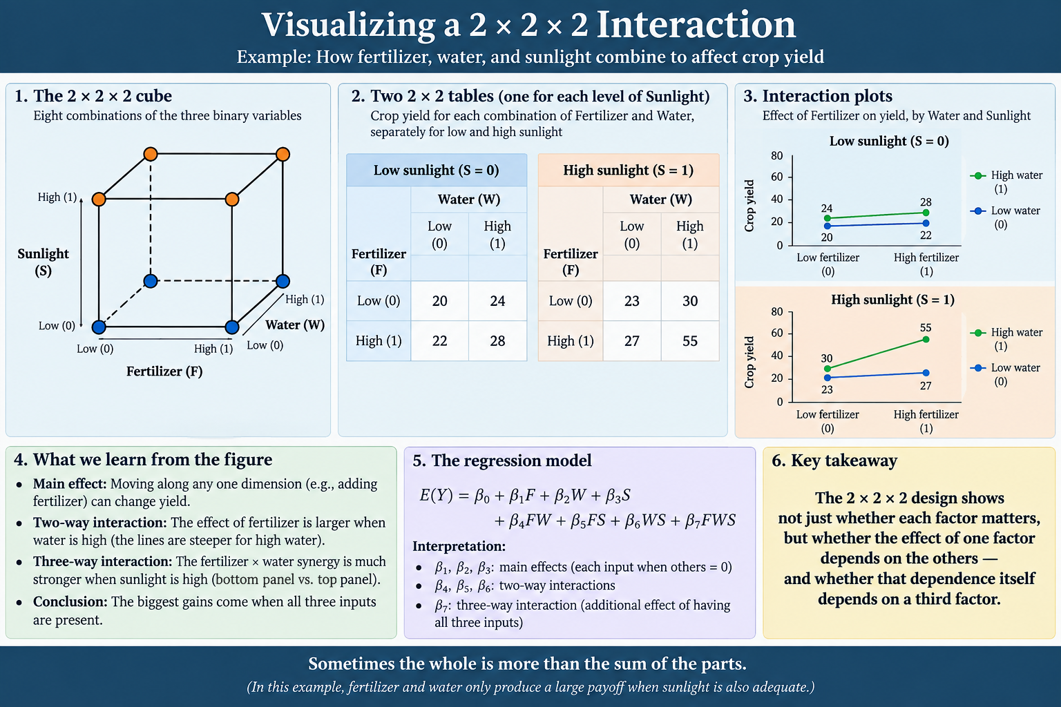
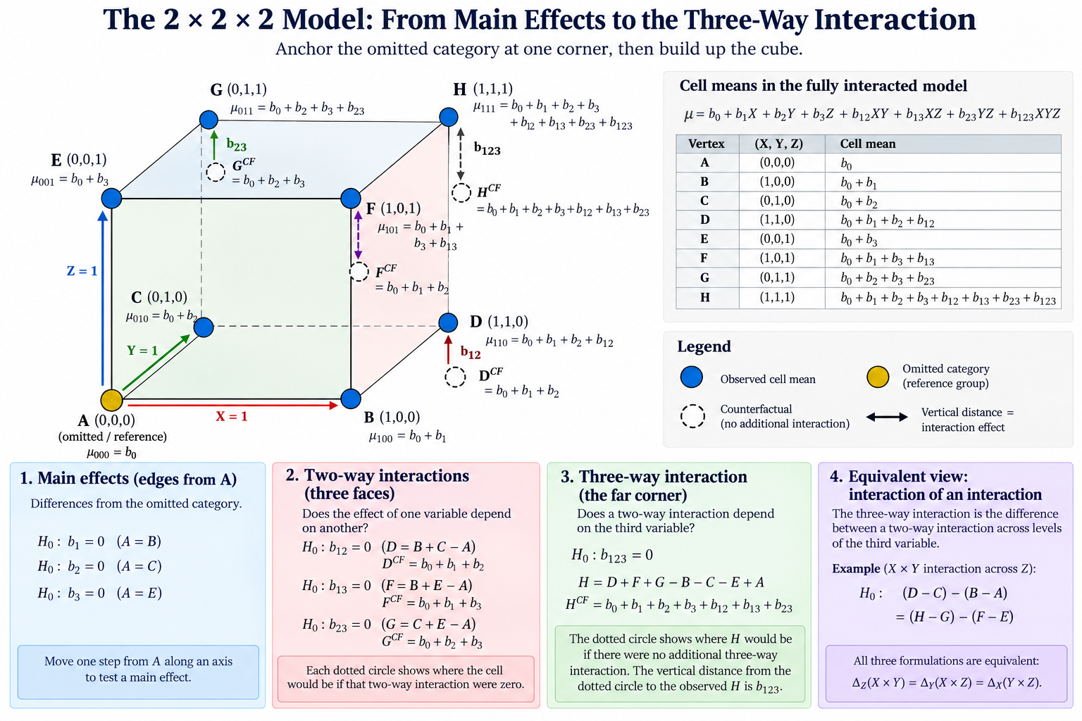
Dummy variables let a regression compare groups, and interaction terms let the effect of a variable differ from one group to another. Together they turn a single model into a set of hypothesis tests about differences in intercepts and slopes.
Covers the errors that come from fitting the wrong functional form, including non-linear relationships and highly leveraged outliers, and the quadratic and log models that fix them. Also shows the distinct signatures of measurement error: noise in Y widens confidence intervals, while noise in X biases the slope toward zero.
Consolidates the seven main threats to regression inference, from selection and omitted variables to multicollinearity and simultaneity. Statistical power asks the mirror-image question: whether a study could have detected a real effect in the first place.
Part 2 — Research Design and Counterfactuals
Every causal claim implies a counterfactual, the outcome that would have occurred without the program, and research design is the work of building a credible stand-in for it. A school district's suicide rate looks high, average, or low depending on which comparison group is chosen.
Tests whether treatment and comparison groups are comparable, using balance tables, attrition checks, and the Bonferroni correction. Introduces the three counterfactual estimators and the assumption each requires, then defines effect sizes and statistical power for research design.
Most outcomes that public programs care about are latent constructs that can only be measured through an instrument, so an estimate is only as good as its measures. Covers validity, reliability, Cronbach's alpha, weighted indices built with factor analysis, and the politics of performance metrics.
Evaluates a study's internal validity as a structured search for competing explanations of its results. Each of the ten Campbell Score items is a rival hypothesis that must be ruled out, with selection and attrition treated as guilty until proven innocent.
Two chapters evaluate the same school choice program with the same data and reach opposite conclusions. Scoring both studies shows that the choice of comparison group and estimator, not the data, drives the difference.
A synthesis unit that estimates program impact three ways, reflexive, post-test only, and difference-in-difference, on the same cognitive-ability study. The work is interpretation: identify the counterfactual behind each model, test its assumptions, and defend the estimate you believe.
Part 3 — Regression Tools for Impact Analysis
Models a single unit observed many times before and after an intervention, separating the pre-existing trend from what the policy changed. The model distinguishes an immediate change in level from a sustained change in slope, and checks the residuals for autocorrelation.
Recasts the difference-in-difference estimator as a regression, where the coefficient on a group-by-period interaction is the program effect. The groups need not be equivalent at baseline, but they must have been trending in parallel before the intervention.
With repeated observations on the same units, fixed effects give each unit its own intercept, so nothing stable about a unit can confound the estimate. Compares pooled, random effects, and fixed effects specifications, and the tests that guide the choice among them.
When the policy variable is correlated with the error term, OLS is biased no matter how much data you have. An instrument that moves the treatment but affects the outcome only through it recovers the effect, built step by step with two-stage least squares.
When eligibility depends on crossing a cutoff, units just above and just below the threshold are nearly comparable, and the jump in outcomes at the cutoff is the program effect. The design is highly credible but local: it says little about units far from the threshold.
For yes-or-no outcomes, logistic regression keeps predicted probabilities between 0 and 1, at the cost of coefficients reported in log-odds. Converting to probabilities shows that the same change in X is worth different amounts depending on the starting point.
Builds a comparison group from observational data by pairing each treated unit with untreated units that had a similar probability of treatment. Matching can only balance what was measured, so it addresses selection on observables alone.