Unit 01
Nuts and Bolts of Regression
Slopes, intercepts, residuals, and what a regression line actually claims.
The building blocks of a bivariate regression model: sample variance and standard deviation, the slope, the intercept, the regression line, and the error term.
Before we can talk about causal impact we need a model that describes the relationship between a treatment and an outcome. The running example asks whether caffeine intake raises heart rate — a question that is easy to model and hard to interpret, which makes it a good place to start.
-
Learning objectives
- Explain what a regression slope represents (a conditional mean).
- Write down and apply the formulas for the regression coefficients.
- Tabulate residuals and decompose the total sum of squares.
Lectures & Notes
Building a Regression Model
Caffeine and heart rate, from scatterplot to fitted model to residual table.
Total Sum of Squares Decomposition
Where the variance of Y goes once a model is fit — SST, SSE, and SSR.
Lab & Template
Lab P101 — Regression Review
Calculate a bivariate slope and intercept by hand on five data points, tabulate residuals, and compute R-squared. Worked on paper rather than in R.
Reference Material
- Using Regression Models to Estimate Program Effects Reichardt, C. S., & Bormann, C. A. (1994). Handbook of Practical Program Evaluation.
- Applied Regression: An Introduction Lewis-Beck, C., & Lewis-Beck, M. (2015). Sage. Reference for the core formulas.
- OpenIntro Statistics, Ch. 8 — Introduction to Linear Regression Diez, D. M., Barr, C. D., & Cetinkaya-Rundel, M. (2012).
- Regression Review Self-Test Benchmark your baseline knowledge before starting the sequence.
- Common Statistics Notation One-page key to the symbols used throughout the lectures.
Unit 02
Variance, Standard Errors, and Confidence Intervals
How much of your estimate is signal, and how far off is it likely to be?
Confidence intervals are built from standard errors, standard errors are built from residuals, and residuals come out of the regression model. This unit walks that chain backwards until the whole apparatus of hypothesis testing rests on quantities you can calculate by hand.
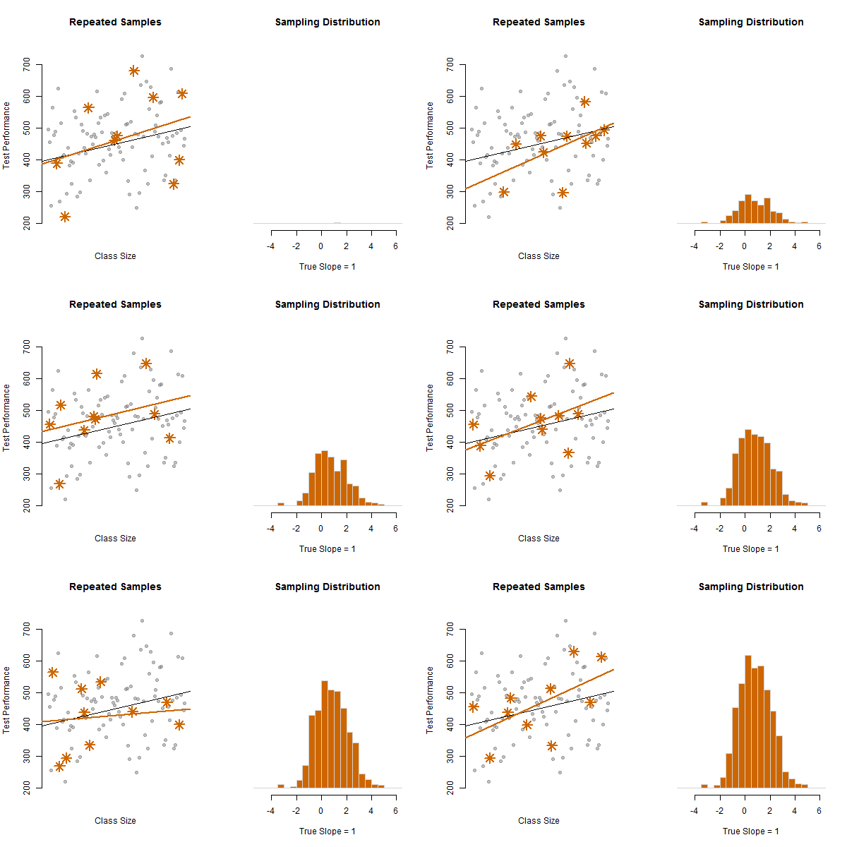
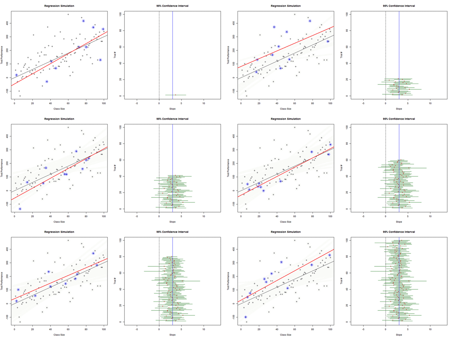
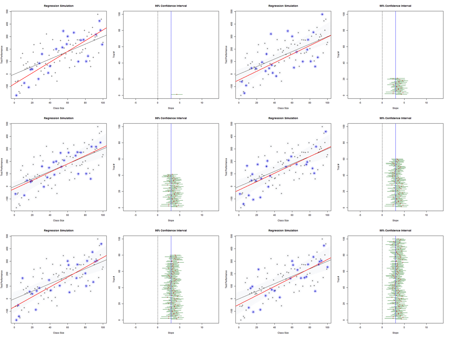
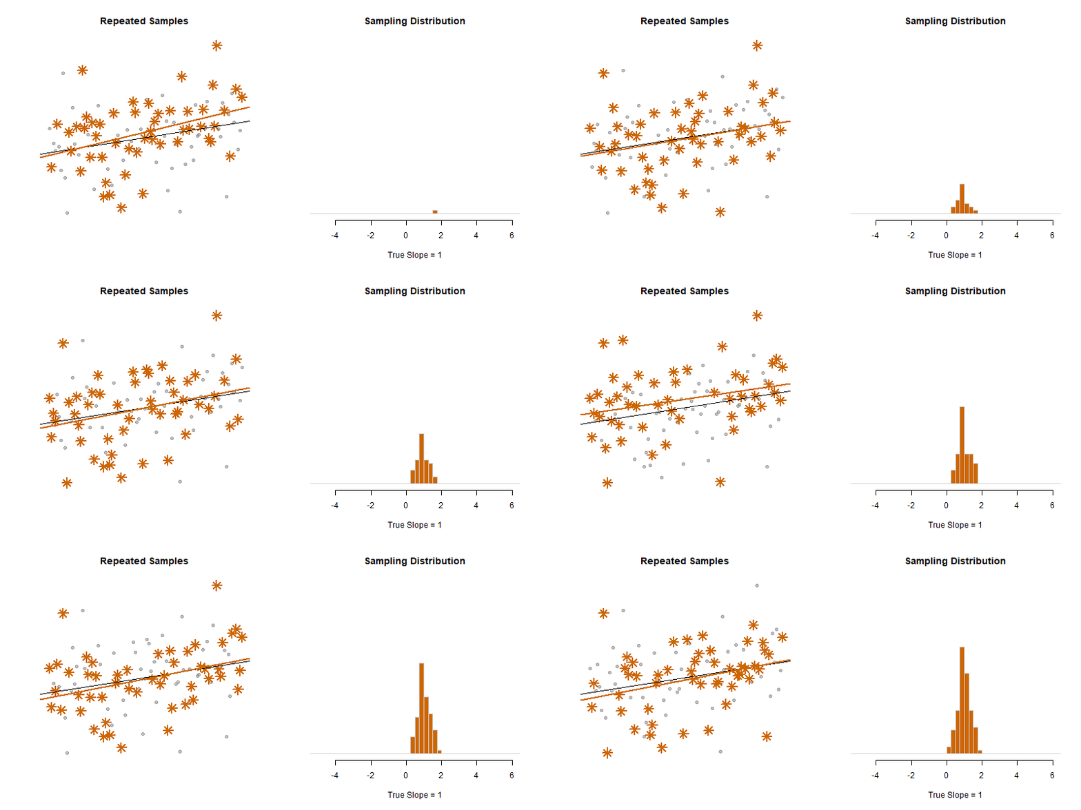
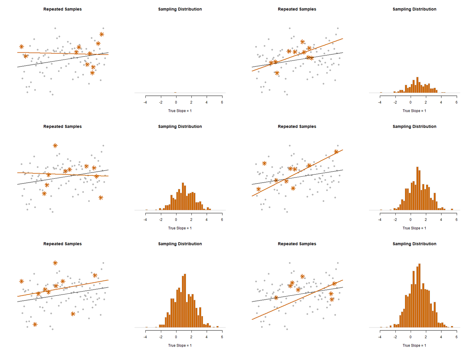
The distinction that does the most work here is between the distribution of the sample (how spread out your data are) and the sampling distribution (how spread out your estimates would be across repeated samples). Standard deviation describes the first; standard error describes the second.
-
Learning objectives
- Build a confidence interval around a slope estimate of program impact.
- Distinguish standard deviation from standard error, and totals from averages.
- Read a regression table reporting several models side by side.
Lectures & Notes
Variance, Covariance, and the Regression Slope
Everything in this lecture is built from one quantity — the deviation from the mean.
Partitioning the Variance of Y
Explained versus unexplained variance, and what R-squared is measuring.
Standard Error of the Slope
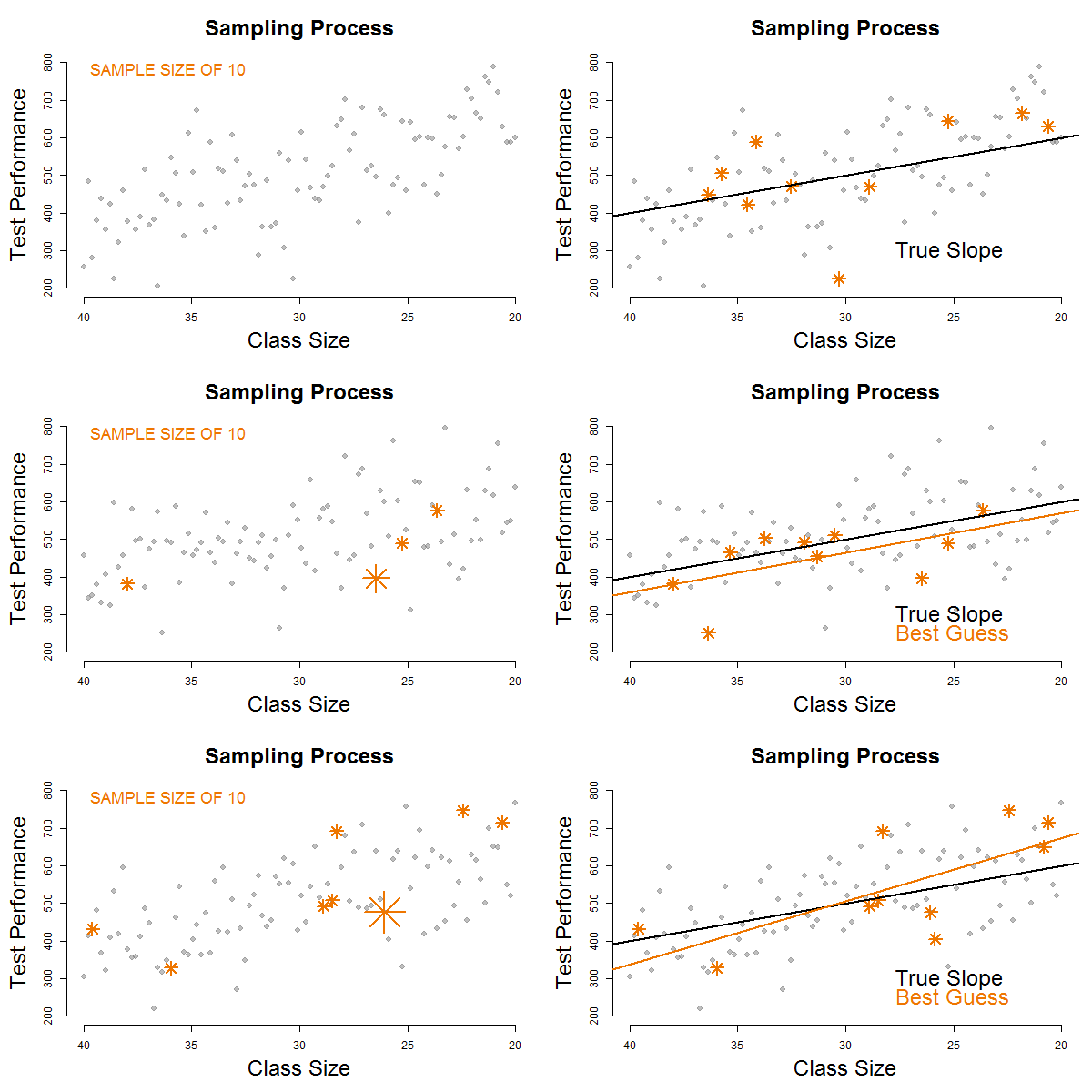
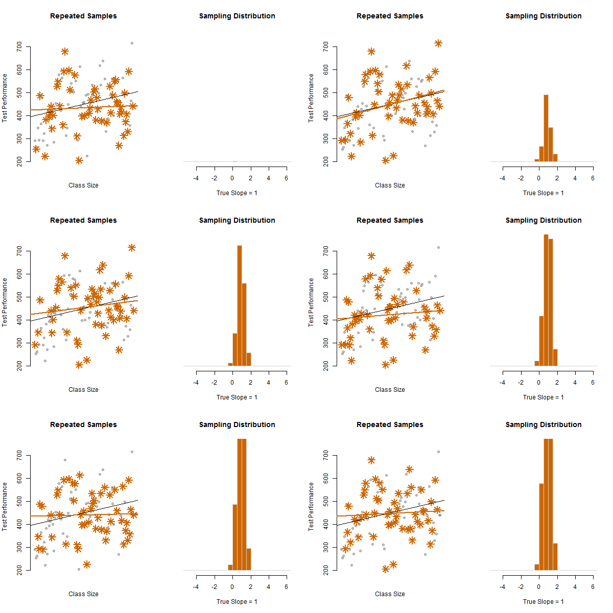
The three levers — residual variance, spread of X, and sample size.
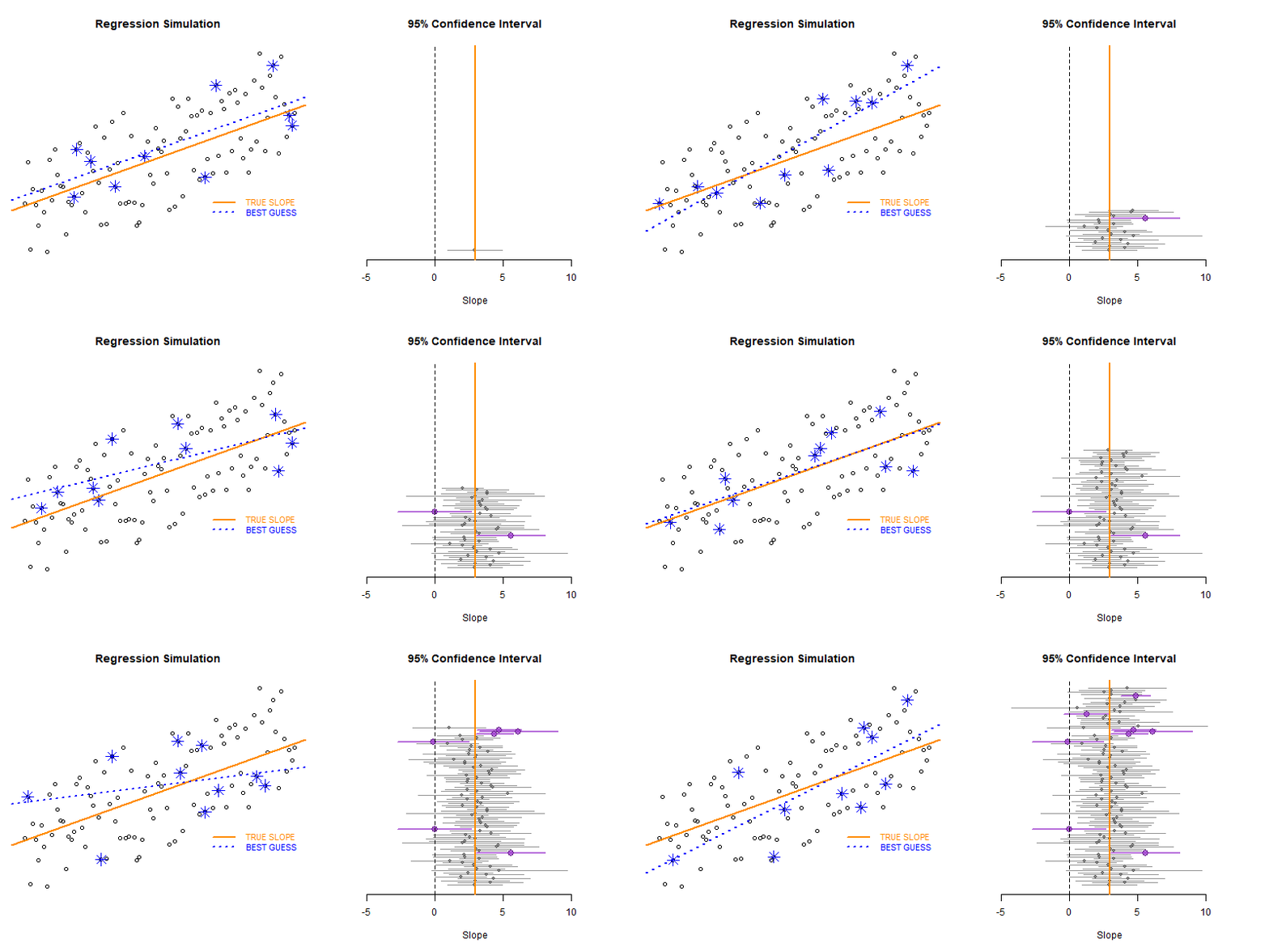
Animations (3)
Confidence Intervals
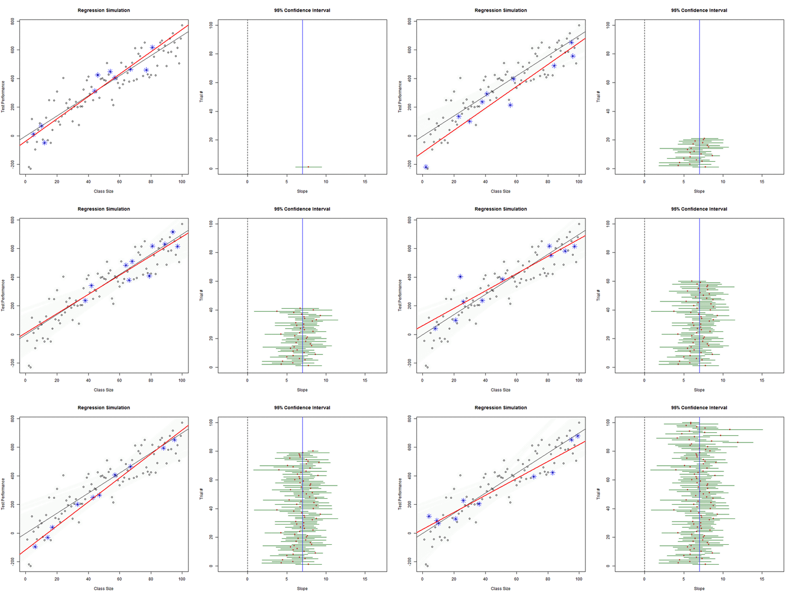
Turning a standard error into a range of plausible values for the true slope.
Animations (1)
Interpreting Program Impact
Effect size, practical versus statistical significance, and coefficient plots.
Animations (2)
Sample vs. Sampling Distribution
A short reading guide on the distinction students most often collapse.
Animations (3)
Lab & Template
Lab P102 — Class Size and Confidence Intervals
Opens the education-policy case study used for the rest of the sequence. Build confidence intervals around slope estimates and run visual hypothesis tests with coefficient plots.
Reference Material
- Common Statistics Notation Symbol key — worth keeping open while working through these lectures.
- The New Statistics, Ch. 1 Estimation, effect sizes, and why p-values are not the whole story.
- The New Statistics, Ch. 2 Confidence intervals as the primary reporting unit.
Unit 03
Control Variables
Two kinds of control variable, and the two different things they do to a model.
Moving from bivariate to multiple regression: Y = b0 + b1*X1 + b2*X2 + e, where X1 is
always the policy variable and everything after it is a control.
Some controls are correlated with the outcome but not with the treatment — they shrink standard errors and buy precision. Others are correlated with both — they move the slope. Knowing which kind you have added is the difference between a more efficient model and a different answer. Ballentine Venn diagrams are introduced here as the tool for keeping the two straight.
-
Learning objectives
- Predict how adding a given control will change the slopes in a model.
- Predict how adding a given control will change the standard errors.
- Use Ballentine diagrams to compare competing specifications.
Lectures & Notes
Control Variables
What a control variable does to the slope, and what it does to precision.
Control Variables in R
Worked example with regression tables and partial-effect scatterplots.
Lab & Template
Lab P103 — Control Variables
Model code is provided; the work is interpretation. Compare specifications on the class-size data and explain what each control is doing to the estimate.
Reference Material
- Multiple Regression Tufte, E. R. (1974). Data Analysis for Politics and Policy, Ch. 4.
Unit 04
Omitted Variable Bias
The variable you left out is still in the model — it is hiding in your slope.
When a variable that belongs in the model is left out, its effect does not disappear.
It gets absorbed into the coefficients of the variables that remain, in an amount you
can calculate exactly: bias = a1 * B2, where a1 comes from the auxiliary regression
of the omitted variable on the policy variable.
The canonical example is the 1989 “crack baby” research, where a strong apparent effect of prenatal cocaine exposure on child development largely dissolved once poverty was added to the models. The doctor-patient racial concordance debate is the same story playing out in a current literature.
-
Learning objectives
- Identify variables with the potential to cause omitted variable bias.
- Calculate the size and direction of bias from omitting a variable.
- Explain why randomization breaks the bias term.
Lectures & Notes
Omitted Variable Bias
The full model, the naive model, the auxiliary regression, and the bias term.
A Taxonomy of Control Variables
Confounders, mediators, colliders, and proxies — which to include and which to leave alone.
Randomization Breaks Omitted Variable Bias
Why an experiment sets the auxiliary slope to zero, and what that buys you.
Calculating Bias — Worked Example
Class size and socioeconomic status, with all three regressions run in R.
Indirect Effects Example
Short handout on decomposing an effect that travels through a mediator.
Lab & Template
Lab P104 — Omitted Variable Bias
Estimate the naive model, the full model, and the auxiliary regression on the class-size data, then show that the bias term reconciles the two slopes.
Reference Material
- Crack Babies: Study Ends with Unexpected but Clear Result The omitted variable was poverty. Required reading for this unit.
- Doctor-Patient Racial Concordance — the original study Strong claims from a cross-sectional model.
- Doctor-Patient Racial Concordance — revisited with controls added What happens to the finding once omitted variables enter the model.
- Doctor-Patient Racial Concordance — press coverage The Economist, on why a correction gets less attention than the finding.
Unit 05
Dummy Variables and Interactions
Modeling groups, and testing whether a program works differently for each of them.
Dummy variables are binary 0/1 indicators — one for each level of a categorical variable, minus the reference category:
y = b0 + b1(X) + b2(D) + e
Interactions multiply a covariate by a dummy, which lets the slope itself differ by group:
y = b0 + b1(X) + b2(D) + b3(X)(D) + e
Together they turn a single regression into a set of hypothesis tests about differences between groups — different intercepts, different slopes, or both.
-
Learning objectives
- Construct dummy variables and choose a sensible reference category.
- Interpret main effects and interaction terms in the same model.
- State and test hypotheses about group differences in intercepts and slopes.
Lectures & Notes
Interactions in Regression Models
How a single interaction term changes the meaning of every other coefficient.
Hypothesis Testing with Dummy Variables
Which coefficient answers which question about group differences.
Three Counterfactual Estimators
Pre-post, post-only, and difference-in-difference — each written as a dummy variable regression.
Groups in Regression Models
The R-side treatment — building dummies, setting factor levels, reading output.
Lab & Template
Lab P105 — Dummy Variables and Group Hypotheses
Construct group indicators, fit models with and without interaction terms, and use the coefficients to test explicit hypotheses about group differences.
Reference Material
- Regression with Interaction Effects — practice questions Work these before the lab.
- Regression with Interaction Effects — solutions Check your answers here.
- Interaction Effects in Research Background on why interactions are so often misread.
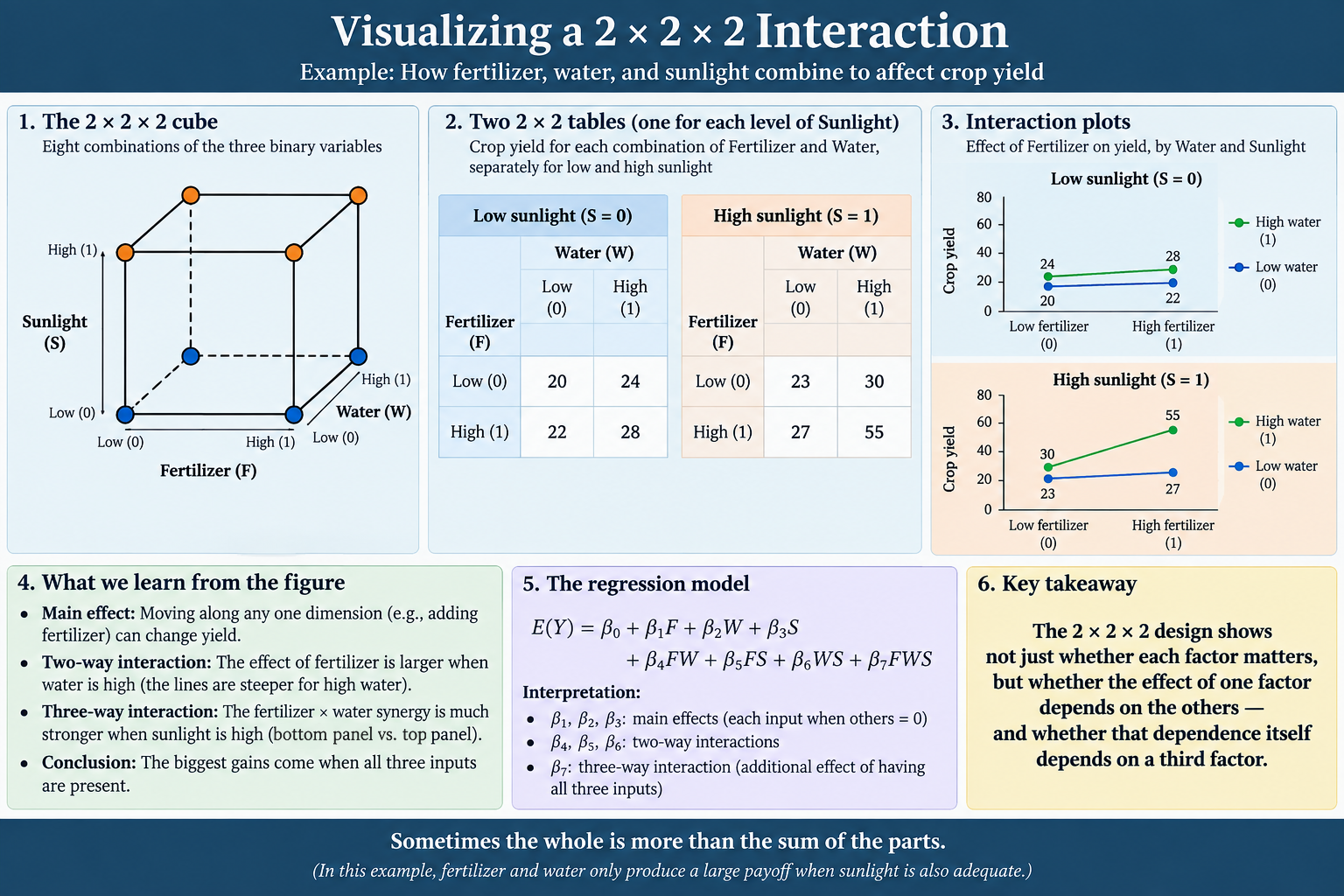
- Visualizing a 2 × 2 × 2 Interaction One-page graphic. Fertilizer, water, and sunlight as cell tables, interaction plots, and a fully interacted regression.
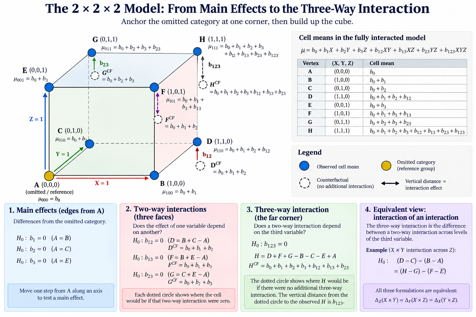
- The 2 × 2 × 2 Model: From Main Effects to the Three-Way Interaction One-page graphic. Maps every coefficient to a corner of the cube and the hypothesis test it answers.
Unit 06
Specification and Measurement Error
What goes wrong when you run the regression without looking at the data.
Specification bias is the error you get from fitting the wrong functional form — a straight line through a curved relationship, or a slope dragged around by a highly leveraged outlier. Because OLS minimizes squared error, a residual twice as large has four times the influence, which is why outliers near the extremes of X do so much damage.
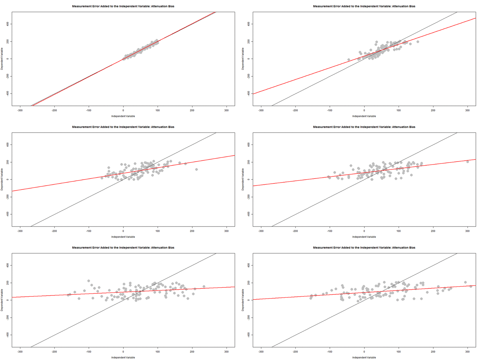
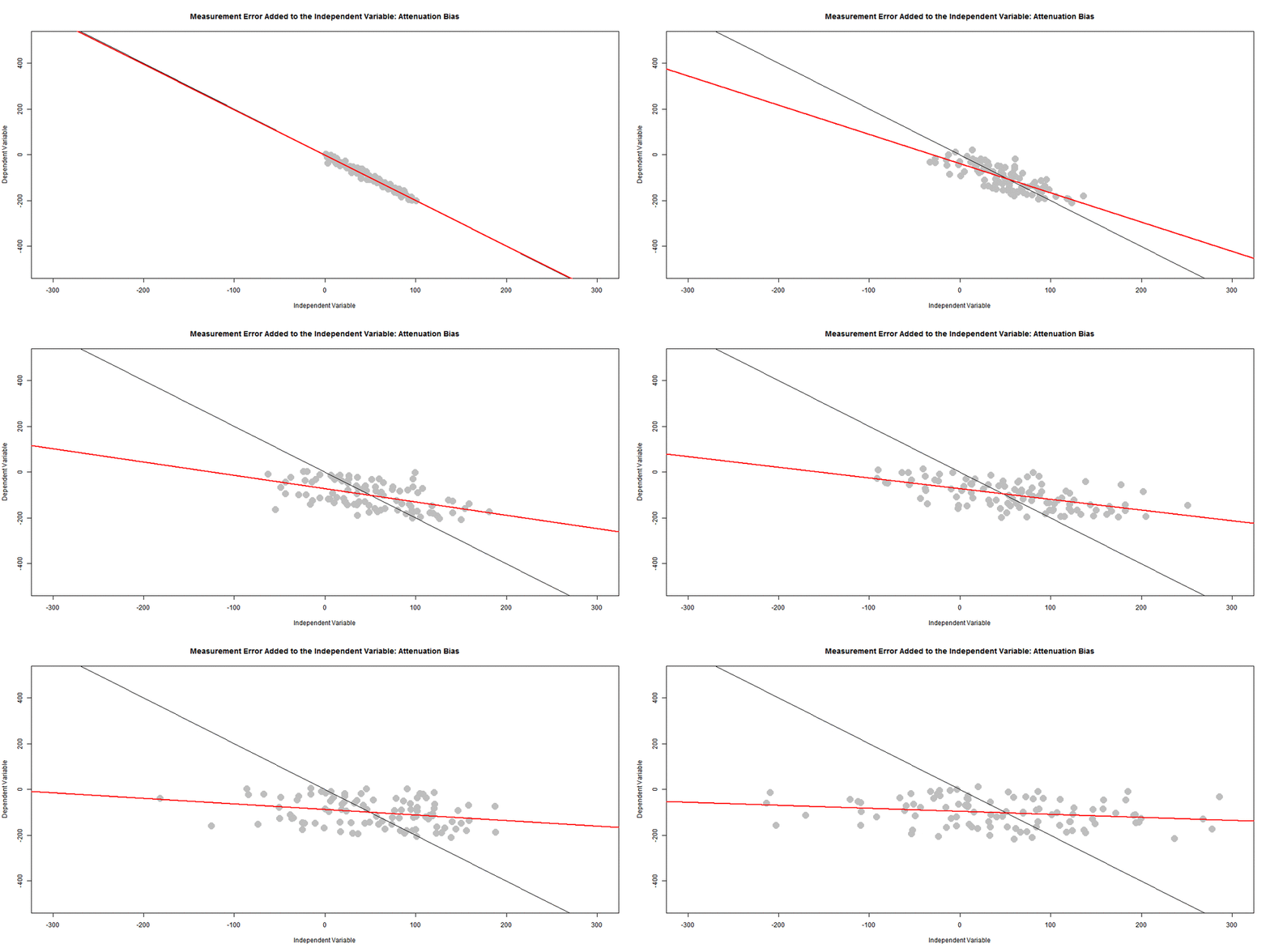
The fixes are quadratic terms for non-linearity and log transformations for skew and for modeling growth rates rather than levels. Measurement error is the companion problem: error in the dependent variable inflates standard errors, while error in the independent variable attenuates the slope toward zero.
-
Learning objectives
- Diagnose specification bias from residual plots rather than from summary statistics.
- Identify leveraged outliers and run sensitivity analysis on them.
- Specify and interpret quadratic and logged regression models.
Lectures & Notes
Bias from Specification or Measurement
Quadratic and log models, plus the distinct signatures of measurement error in X and Y.
Animations (3)
Lab & Template
Lab P106 — Non-linear Models
Fit and interpret a quadratic regression and a logged regression, and report the marginal effect at meaningful values of X.
Reference Material
- Anscombe's Quartet Four datasets, identical regression output, four completely different stories.
- Marginal Effects in Quadratic Regression Models How to report a slope that changes across the range of X.
- Interpreting Logged Regression Models Log-linear, linear-log, and log-log specifications side by side.
Unit 07
Threats to Inference and Statistical Power
The seven ways a regression lies to you, and whether your study could detect anything at all.
A consolidated tour of the things that corrupt a regression inference: selection, omitted variable bias, measurement error, specification, group heterogeneity, multicollinearity, and simultaneity. Most of the sequence so far has been a slow walk through the middle of that list; this unit puts the whole set in one place.
Statistical power is the mirror-image question. Before asking whether a program worked, ask whether the study was ever capable of showing that it worked — a null result from an underpowered design carries almost no information.
-
Learning objectives
- Name the mechanism behind each of the seven threats and its signature in the output.
- Diagnose which threat is most plausible in a given study design.
- Assess whether a design has enough power to detect an effect worth detecting.
Lectures & Notes
Seven Sins of Regression
Selection, omitted variables, measurement error, specification, heterogeneity, multicollinearity, simultaneity.
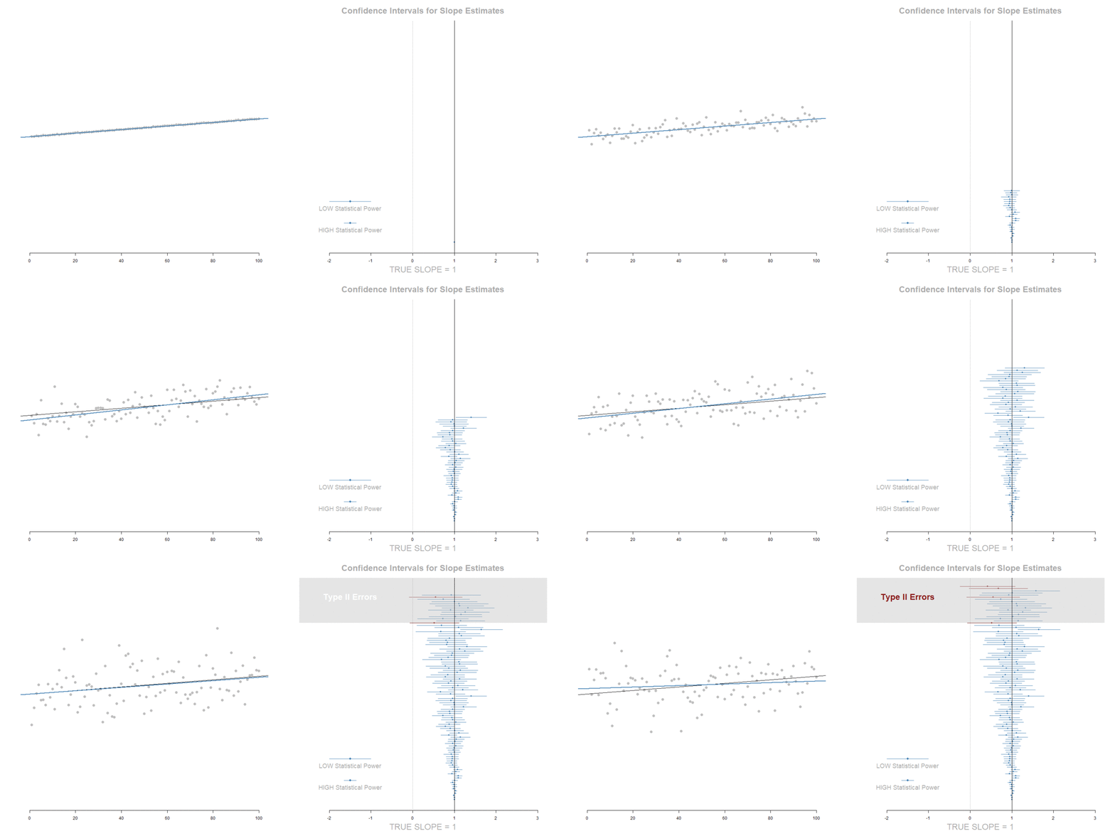
Statistical Power
Effect size, sample size, and the probability of detecting an effect that is really there.
Animations (3)
Reference Material
- Seven Sins of Regression Analysis Concise one-page summary of all seven threats.
- Difference-in-Difference Models One design-based route around several of the seven.
Unit 08
Counterfactual Analysis
The world that did not happen, and why choosing it decides your answer.
A causal claim is a counterfactual claim in disguise: to say the program caused the outcome is to say the outcome would not have occurred without it. Since we only get one world, we build comparison groups that stand in for the one we cannot observe.
The running example is a suburban California school district with an unusual number of student suicides. Tested against the state population it looks high; against all high school students it looks average; against suburban high school students it looks low. Same data, same model, three defensible counterfactuals, three opposite conclusions.
-
Learning objectives
- Define a counterfactual and explain why every causal claim implies one.
- Identify the comparison group hiding inside any null hypothesis.
- Distinguish a comparison group from a control group.
- Construct the elements of a randomized control trial and check they were implemented correctly.
Lectures & Notes
Introduction to Counterfactual Analysis
Lewis on subjunctive conditionals, the treatment effect as a difference of means, and five examples where the comparison group decides the result.
Contrasts and Effect Size
One staggered-start study read four different ways — dosage, pooling, and the age confound.
Lab & Template
Lab P201 — Counterfactual Reasoning with RCTs
Read the Bingham & Felbinger cognitive-ability study and report on the control group, the program theory, the treatment and its duration, and the confounding factors.
Reference Material
- Improving Cognitive Ability in Chronically Deprived Children (Ch. 5) Bingham & Felbinger, Evaluation in Practice. The RCT case study used in Lab P201.
- Causal Inference Based Upon Counterfactuals Background on the potential-outcomes framework.
- An Introduction to Causal Inference Elwert. Graphical models and the logic of confounding.
- Using Regression Models to Estimate Program Effects Reichardt & Bormann (1994). Carried over from the first course.
Unit 09
Testing and Varieties of the Counterfactual
Selection, attrition, balance tests, and the three estimators you can build.
Two lectures that belong together. The first asks whether your groups are comparable at all — the selection problem, non-random attrition, and the balance table that every study should report. The second asks what to compute once they are: the reflexive, post-test-only, and difference-in-difference estimators.
The organizing insight is that diff-in-diff is the general case. Reflexive is valid only when there is no secular trend; post-test-only is valid only when the groups were equivalent at baseline. Each of the weaker estimators is a bet that one term drops out.
-
Learning objectives
- Explain why participants differ from non-participants, and what randomization or matching fixes.
- Apply the Bonferroni correction to a table of contrasts and decide whether groups are equivalent.
- Distinguish random from non-random attrition and run the tests that tell them apart.
- Compute all three estimators and state the identifying assumption each one needs.
Lectures & Notes
Testing the Validity of the Counterfactual
The selection problem, the microfinance table, attrition, unhappy randomization, and the Bonferroni correction.
Varieties of the Counterfactual
Three estimators, the parallel-lines assumption, and the gender pay gap worked example.
Effect Size: ATE, ITT, and TOT
What counts as an effect, and the difference between being offered a treatment and taking it.
Animations (3)
Statistical Power and Research Design
A consolidated design deck that closes on power — what shrinks a confidence interval, and why both sample size and effect size move it.
Animations (3)
Happy Randomization
Short companion piece on why balance fails 5% of the time by construction.
Lab & Template
Lab P202 — Tests for Group Equivalence
Build a balance table, apply the corrected decision rule, and decide whether the randomization in a study can be called happy.
Reference Material
- A Dialogue with Tom Cook and Michael Scriven Cook, Scriven, Coryn & Evergreen (2010). Contemporary thinking about causation in evaluation.
- A Review of Quasi-Experimental Design Where quasi-experimental methods sit relative to the randomized trial.
- Alternatives to Randomized Control Trials When an RCT is impractical or unethical, and what replaces it.
- Examples of Quasi-Experiments in Public Health Worked designs from the health literature.
Unit 10
Measurement Theory
Before you estimate an effect, make sure the number measures the thing you care about.
Every estimator in this course takes the outcome variable on faith. Measurement theory is where that faith gets checked. Two Manhattan neighborhoods can post the same poverty rate while one is trapped in inter-generational poverty and the other is a way station for upwardly mobile immigrant families — same number, different construct.
Some things can be counted directly. Most of what public programs care about — health, happiness, depression, social capital — are latent constructs that can only be measured through an instrument: a survey scale, a coding protocol, a standardized exam. An instrument is valid if it measures the construct it claims to, and reliable if its items measure that construct consistently. Cronbach’s alpha is the workhorse statistic for the second question, and a scale can often be improved by dropping the item that does not belong.
The unit closes with the politics of measurement: once a metric is tied to rewards and penalties, people start managing the metric instead of the outcome.
-
Learning objectives
- Distinguish direct measures, markers or proxies, and latent constructs.
- Explain the difference between measurement validity and measurement reliability.
- Calculate and interpret Cronbach's alpha, and use item correlations to improve a scale.
- Build weighted composite indices with factor analysis, and explain how it differs from PCA.
- Identify the perverse incentives that performance metrics can create.
Lectures & Notes
Measurement Theory
What the poverty rate hides, the three types of measures, and Cronbach's alpha on the good-dancer and bro-culture scales.
Signal, Noise, and Reliable Indices
Short lecture note: M = T + e, reliability as a signal-to-noise ratio, and how experts build indices of neighborhood quality.
Weighted Composite Indices
More detail: why weighting items by loading and noise beats a simple average, with the optimal weights and a worked example.
R Walkthroughs
Factor Analysis
Reduce 30 census variables to four named neighborhood constructs: factorability checks, parallel analysis, loadings, a Heywood case, and factor scores compared against a simple index.
PCA versus Factor Analysis
Fit both methods to the same data, line up the dimensions, and compare loadings, communalities, and scores to see where total variance and common variance part ways.
Lab & Template
Measurement Lab — A Community Well-Being Index
Do the warm-up, then use Census data on the Index Design tab to pick 5 of 30 candidate variables for an index of community well-being. The index must reach a Cronbach's alpha of at least 0.70.
Reference Material
- Measurement Theory and Practice Aparasu, R. R. (2011). Research Methods for Pharmaceutical Practice and Policy, Ch. 4. Levels of measurement, reliability, and validity.
- Construct Measurement and Validation Procedures in MIS and Behavioral Research MacKenzie, Podsakoff & Podsakoff (2011). MIS Quarterly, 35(2). The full scale-development process, from conceptual definition to validation.
- Forget the Myers-Briggs, Use the Big Five Kelly (2019). HeadStuff. A popular instrument that fails the test-retest reliability standard.
- Punishing and Toxic Neighborhood Environments Predict Social Mobility Manduca & Sampson (2019). PNAS. What neighborhood measures add beyond the concentrated poverty rate.
- Management Accounting & Control Scales Handbook Schäffer (2007). A reference catalogue of published multi-item scales — look here before writing your own.
Unit 11
Campbell Scores
Ten competing hypotheses that could explain your result instead of the program.
A framework for evaluating the internal validity of a study as a structured search for competing hypotheses. The program hypothesis says the change came from the program; each Campbell Score item is a rival explanation that has to be ruled out first.
The scoring rule is asymmetric on purpose. Selection and non-random attrition are so common in observational work that they are guilty until proven innocent — a study must show it handled them. The remaining eight items are innocent until proven guilty: you have to argue from evidence in the study that the threat is live.
-
Learning objectives
- Identify design weaknesses that threaten internal validity and could undermine results.
- Read an evaluation study efficiently by knowing which tests the author owes you.
- Score a study on all ten items and defend each score with evidence.
- Package a description of your own research design so that others can assess it.
Lectures & Notes
Campbell Scores: Eliminating Competing Hypotheses
The ten items, the two standards of proof, and the fix for each threat.
Lab & Template
Lab P203 — Scoring Three Studies
Score Chapters 7, 8, and 11 on every Campbell Score item, awarding +1 where the threat is adequately neutralized and +0 where it is not, with reasoning for each.
Reference Material
- Post-Test Only Estimator (Ch. 7 — hospital follow-up care) Bingham & Felbinger. One of the three studies scored in Lab P203.
- Pre-Post with Comparison (Ch. 8 — energy savings) Bingham & Felbinger. Second study scored in Lab P203.
- Reflexive Study Design (Ch. 11 — nutrition behavior change) Bingham & Felbinger. Third study scored in Lab P203.
- A Checklist for Classifying Health Intervention Studies A parallel framework from the health literature.
Unit 12
Two Studies, Same Data, Opposite Conclusions
A riddle in two chapters, and the estimator choice that resolves it.
Chapters 20 and 21 evaluate the same school choice program using the same data and reach opposite conclusions: Chapter 20 finds the program ineffective, Chapter 21 finds it effective. Nothing about the data changed.
Two things differ. Chapter 21 uses a strong counterfactual where Chapter 20 uses a weak comparison group — and, more importantly, each chapter calculates program effects with a different estimator. Work out which of the three each author used and the divergence stops being mysterious.
The time-frame question is subtler than it looks. If a study collects four years of data but analyses only one, its time-frame is one year, not four. Here the time-frame is a function of how effects are calculated, not of how long collection ran.
-
Learning objectives
- Reverse-engineer which counterfactual estimator a published study actually used.
- Explain how estimator choice alone can flip a conclusion about program effectiveness.
- Define a study's analytic time-frame separately from its data collection window.
Lectures & Notes
No new lectures this unit
The exercises draw on the counterfactual and Campbell Score material already covered. The four decks below are the ones you will need at hand.
Lab & Template
Lab P204 — Campbell Scores on Competing Studies
Apply the Campbell Score to both school choice chapters and explain why two skilled research teams reached different conclusions from identical data.
Reference Material
- Evaluation of a School Choice Program (Ch. 20 and Ch. 21) Bingham & Felbinger. Focus on Tables 10A–10D and the regression models in 11A and 11B.
- Pre-Post with Control (Ch. 5) Companion chapter for comparing designs.
Unit 13
Comparing the Three Estimators on One Dataset
Run all three, test the assumptions, and defend the one you believe.
The synthesis lab. Return to the cognitive-ability study from Unit 08 and calculate program impact three ways — reflexive, post-test only, and difference-in-difference — on the same data.
The regression models are provided. The work is interpretation: read the coefficients correctly, identify which counterfactual each model deploys, run the identification tests, and decide which estimates you actually believe. Some estimators are valid in this context and some are not.
-
Learning objectives
- Map a fitted regression back to the counterfactual it implements.
- Run identification tests and check whether each estimator's assumptions hold.
- Argue in writing for one estimate over the others.
Lectures & Notes
The Three Counterfactual Estimators
The reference for this lab — formulas, assumptions, and the parallel-lines test.
Lab & Template
Lab P205 — Difference-in-Difference
Compare program effects across all three estimators on one dataset, check the assumptions behind each, and write up which you trust and why.
Reference Material
- Improving Cognitive Ability in Chronically Deprived Children (Ch. 5) The same study from Lab P201, now analysed rather than described.
- Designing Difference-in-Difference Studies Wing, Simon & Bello-Gomez (2018). Best practices for public health policy research.
Unit 14
Interrupted Time Series
One group, many time points, and a policy that lands in the middle of them.
The reflexive counterfactual with enough time points to see a trend. A single unit is observed repeatedly before and after an intervention, and the model separates the pre-existing trajectory from what the intervention changed.
Y = b0 + b1·T + b2·D + b3·P + e, where T counts time, D is a treatment dummy
(0 before, 1 after), and P counts time since the intervention. That gives b1 as the
pre-intervention trend, b2 as the immediate level change, and b3 as the sustained
change in slope. A policy can have an immediate effect, a sustained effect, both, or
neither, and the four coefficients tell them apart.
-
Learning objectives
- Recognize when data are suited to an interrupted time series model.
- Organize a dataset into the time, treatment, and time-since-treatment variables the model needs.
- Interpret each coefficient and identify the two counterfactuals in the model.
- Detect and test for autocorrelation in the residuals.
Lectures & Notes
Interrupted Time Series
Tobacco taxes, the Oklahoma City birth-rate series, counterfactual prediction at each time point, and the Durbin-Watson test.
Lab & Template
Lab P301 — Interrupted Time Series
Build the three time variables, fit the model, and plot predicted outcomes against their counterfactuals.
Reference Material
- Rent Control as a Time Series (Ch. 12) Bingham & Felbinger. A worked interrupted time series in policy.
- NYC Robberies Occur as School Gets Out A seasonality and cycle example worth reading alongside the lecture.
Unit 15
Difference-in-Difference Models
The strong counterfactual, now as a regression rather than a table of four means.
The estimator introduced in Unit 09 becomes a regression here. Two groups, two periods, and an interaction term whose coefficient is the program effect: the treated group’s change minus the comparison group’s change.
Its strength is that the groups need not be equivalent at baseline — level differences difference out. What it does require is that the two groups were moving in parallel before the intervention, which is a testable claim whenever you have more than one pre-period.
-
Learning objectives
- Specify a difference-in-difference model as an interaction in regression.
- Read the program effect off the interaction coefficient.
- State and test the parallel trends assumption.
Lectures & Notes
Difference-in-Difference Models
The four means, the interaction specification, and what breaks when trends are not parallel.
Lab & Template
Lab P302 — Difference-in-Difference
Fit the interaction model, interpret the effect, and check the pre-treatment trends.
Reference Material
- Designing Difference-in-Difference Studies Wing, Simon & Bello-Gomez (2018), Annual Review of Public Health.
- Impact Evaluation in Practice, Ch. 7 Gertler et al. (2016), World Bank. Difference-in-differences.
- Shutdowns Prevented 60 Million Coronavirus Infections A high-profile diff-in-diff style policy claim to read critically.
Unit 16
Panel Data with Fixed Effects
Let every unit keep its own intercept, and identify the effect from within-unit change.
With repeated observations on the same units, a fixed effects model gives each unit its own intercept and estimates the slope from variation within units over time. Anything stable about a unit — however unmeasurable — is absorbed and can no longer confound the estimate.
The lecture contrasts the pooled model, where every unit shares one intercept, with the random effects and fixed effects alternatives, and shows the equivalence between the dummy-variable formulation and the demeaned-data formulation.
-
Learning objectives
- Explain what a unit fixed effect absorbs and what it cannot.
- Compare pooled, random effects, and fixed effects specifications on the same panel.
- Fit a fixed effects model both with dummy variables and with the plm package.
Lectures & Notes
Fixed Effect Models
Corn and fertilizer, company R&D investment, pooled vs. grouped intercepts, and the plm package.
Panel Model Specification
Choosing between pooled, random, and fixed effects, and the tests that inform the choice.
Lab & Template
Lab P303 — Fixed Effects
Estimate the same relationship pooled and with fixed effects, and account for the difference.
Reference Material
- Impact Evaluation in Practice (World Bank) Reference text for panel designs.
Unit 17
Instrumental Variables
Borrow the part of your treatment that is uncorrelated with the error.
When the policy variable is correlated with the error term — through omitted variables, measurement error, or simultaneity — OLS is biased and no amount of data fixes it. An instrument is a variable that moves the treatment but affects the outcome only through the treatment.
Two-stage least squares makes the logic explicit: regress the endogenous variable on the instrument, keep the fitted values, and use those in the second stage in place of the original variable.
first.stage  <- lm( x1 ~ z + x2, data=dat )
x1_hat       <- fitted( first.stage )
second.stage <- lm( y ~ x1_hat + x2, data=dat )
-
Learning objectives
- State the two conditions a valid instrument must satisfy.
- Run two-stage least squares by hand and with a canned estimator.
- Compare the full, naive, and IV models and explain the pattern in the slopes.
Lectures & Notes
Instrumental Variables
Endogeneity, the exclusion restriction, and 2SLS built up one regression at a time.
Lab & Template
Lab P304 — Instrumental Variables
Estimate a naive model, build the first stage, and show what the instrument recovers.
Reference Material
- Causal Inference — What If Hernán & Robins. Reference text; the IV chapters are the relevant ones here.
Unit 18
Regression Discontinuity Design
Near an arbitrary cutoff, who gets treated is almost random.
When eligibility is determined by whether a running variable crosses a threshold — a test score, an income line, a date of birth — the units just above and just below the cutoff are close to comparable. The jump in outcomes at the threshold is the effect.
The design buys credibility cheaply, and pays for it in generalizability: the estimate is a local effect at the cutoff, and says nothing about units far from it.
-
Learning objectives
- Identify a running variable and a cutoff in a policy setting.
- Estimate the discontinuity and choose a sensible bandwidth.
- Explain why the estimate is local and what would invalidate it.
Lectures & Notes
Regression Discontinuity Design
The cutoff, the local comparison, bandwidth choice, and what manipulation of the running variable would do.
Lab & Template
Lab P305 — Regression Discontinuity
Fit the discontinuity, vary the bandwidth, and report how sensitive the estimate is.
Reference Material
- Impact Evaluation in Practice, Ch. 5 Gertler et al. (2016). Regression discontinuity design.
Unit 19
Logistic Regression
Binary outcomes, log-odds, and why marginal effects depend on where you stand.
When the outcome is yes/no — admitted, employed, enrolled — the linear probability model can predict probabilities outside [0,1]. The logit link keeps predictions in range at the cost of coefficients that are no longer read directly.
The model reports log-odds, which have to be converted to probabilities before they mean anything. And because the curve is not linear, the value of a change in X depends on the baseline: in the law school admissions example, a 10-point LSAT increase is worth very different amounts starting from 120, from 140, and from 170.
-
Learning objectives
- Explain why a linear probability model is inadequate for a binary outcome.
- Convert log-odds to predicted probabilities.
- Compute marginal effects, centering the other covariates, and interpret them at different baselines.
Lectures & Notes
Logistic Regression
The LPM, the logit link, log-odds to probabilities, and marginal effects across the range of X.
Lab & Template
Lab P306 — Logistic Regression
Fit a logit model, convert coefficients to probabilities, and compare marginal effects at different baselines.
Reference Material
- Reporting Effect Sizes to Facilitate Cumulative Science On reporting effects in a way readers can actually use.
- It's the Effect Size, Stupid Coe. Why the magnitude matters more than the p-value.
Unit 20
Propensity Score Matching
Manufacture a comparison group by pairing each treated unit with its nearest twin.
The post-test-only estimator needs equivalent groups, and observational data rarely supplies them. Matching builds them after the fact: model each unit’s probability of being treated, then pair treated units with untreated units that had similar probabilities.
The lecture works through distance calculations between treated and untreated students, nearest-neighbour matching with and without a caliper, and matching with and without replacement. What matching cannot do is balance anything you did not measure — which is why it addresses selection on observables only.
-
Learning objectives
- Estimate propensity scores with a logit model.
- Apply nearest-neighbour matching and explain the role of the caliper distance.
- Assess balance after matching, and state what matching cannot fix.
Lectures & Notes
Matching
Propensity scores, distance between units, nearest neighbour and caliper rules, and the MatchIt package.
Lab & Template
Lab P307 — Propensity Score Matching
Build matching scores, construct a matched comparison group, and re-estimate the program effect.
Reference Material
- A Review of Quasi-Experimental Design Where matching sits relative to the other quasi-experimental tools.
- The Counterfactual in Program Evaluation Schwartz. Framing reading for the matching approach.