---

---

Current Ratio

Definition & Interpretation

\[Current \: Asset \: Ratio = \frac{Current \: Assets}{Current \: Liabilities}\]

The current ratio is used to measure the overall liquidity of a nonprofit organization.

In its simplest form, it shows how many dollars of current assets an organization has to cover its current obligations. The higher the ratio, the more liquid the organization.

As a rule of thumb, organizations should strive for a current ratio of 1.0 or higher. An organization with a ratio of 1.0 would have one dollar of assets to pay for every dollar of current liabilities.

Variables

Numerator: (Cash + short-term investments + current receivables + inventories + prepaid expenses)

• On 990: (Part X, line 1B) + (Part X, line 2B) + (Part X, line 3B) + (Part X, line 4B) + (Part X, line 8B) + (Part X, line 9B)
  
• SOI PC EXTRACTS: nonintcashend, svngstempinvend,pldgegrntrcvblend, accntsrcvblend, invntriesalesend, prepaidexpnsend
  
• On EZ: Part I, line 22 [cash and short-term investments only]

Denominator: (Accounts payable + grants payable)

• On 990: (Part X, line 17B) + (Part X, line 18B)
  
• SOI PC EXTRACTS: accntspayableend+grntspayableend
  
• On EZ: Not available

Note: This data is only available for organizations that file a full 990, not for EZ filers.

Note: The EZ form only asks filers to report on cash, savings and investments; all receivable accounts, inventories, and prepaid expenses are reported in the line item “other assets” (Part II, line 24), and details are reported in Schedule O. Similarly, the EZ form asks filers to report on total liabilities, with details about payable accounts reported in Schedule O.

liquidity <- ( core$nonintcashend + core$svngstempinvend + 
                         core$pldgegrntrcvblend + core$accntsrcvblend + 
                         core$invntriesalesend + core$prepaidexpnsend )

# can't divide by zero
payables <- ( core$accntspayableend + core$grntspayableend )
payables[ payables == 0 ] <- NA

core$currentratio <-  liquidity / payables
                     
# summary( core$currentratio )

Standardize Scales

Check high and low values to see what makes sense.

x.05 <- quantile( core$currentratio, 0.05, na.rm=T )
x.95 <- quantile( core$currentratio, 0.95, na.rm=T )

ggplot( core, aes(x = currentratio ) ) +  
  geom_density( alpha = 0.5) + 
  xlim( x.05, x.95 )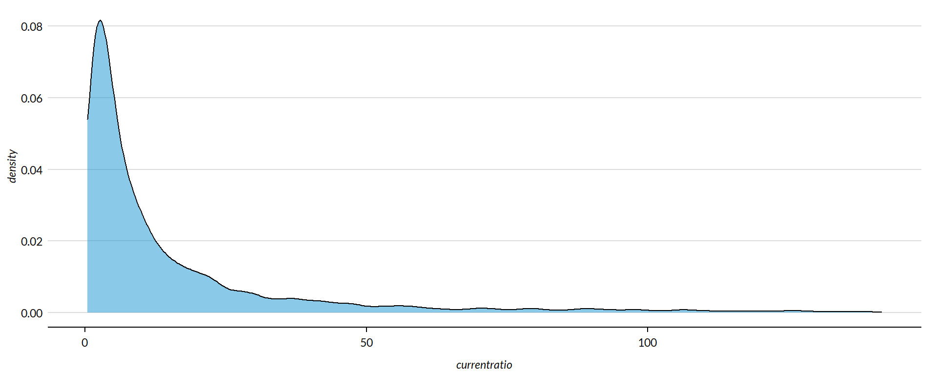 

core2 <- core

# proportion of values that are negative
mean( core2$currentratio < 0, na.rm=T ) 
## [1] 0.002959205
core2$currentratio[ core2$currentratio < 0 ] <- 0

# proption of values above 200% 
mean( core2$currentratio > 200, na.rm=T ) 
## [1] 0.03804692
core2$currentratio[ core2$currentratio > 200 ] <- 200

All values have been capped at the 95th percentile, or 200, to improve readability and exclude outliers. Negative values have been normalized to 0.

Metric Scope

Tax data is available for full 990 filers, so this metric does not describe any organizations with Gross receipts < $200,000 and Total assets < $500,000. Some organizations with receipts or assets below those thresholds may have filed a full 990, but these would be exceptions.

Descriptive Statistics

Convert all monetary variables to thousands of dollars.

core2 %>%
  mutate( # currentratio = currentratio * 10000,
    totrevenue = totrevenue / 1000,
    totfuncexpns = totfuncexpns / 1000, 
    lndbldgsequipend = lndbldgsequipend / 1000,
    totassetsend = totassetsend / 1000,
    totliabend = totliabend / 1000,
    totnetassetend = totnetassetend / 1000 ) %>% 
  select( STATE,  NTEE1, NTMAJ12, 
          currentratio, 
          AGE, 
          totrevenue, totfuncexpns, 
          lndbldgsequipend, totassetsend, 
          totnetassetend, totliabend ) %>%

  stargazer( type = s.type, 
             digits=0, 
             summary.stat = c("min","p25","median",
                              "mean","p75","max", "sd"),
             covariate.labels = c("Current Ratio", "Age", 
                                  "Revenue ($1k)", "Expenses($1k)", 
                                  "Buildings ($1k)", "Total Assets ($1k)",
                                  "Net Assets ($1k)", "Liabiliies ($1k)"))

Statistic	Min	Pctl(25)	Median	Mean	Pctl(75)	Max	St. Dev.
Current Ratio	0	2	6	23	19	200	44
Age	3	22	30	32	41	95	15
Revenue (1k)	-5,377	259	909	4,522	3,672	408,932	14,286
Expenses(1k)	0	263	840	4,192	3,328	382,667	13,466
Buildings (1k)	-4	79	824	3,504	2,868	513,509	13,210
Total Assets (1k)	-7,552	778	2,446	9,262	7,477	672,021	27,039
Net Assets (1k)	-178,870	156	1,094	4,553	4,079	531,068	15,470
Liabiliies (1k)	-2,707	115	816	4,709	3,133	705,623	18,722

What proportion of orgs have a Current Ratio of zero (no outstanding liabilities)?

prop.zero <- mean( core2$currentratio == 0, na.rm=T )

In the sample, 1 percent of the organizations have a Current Ratio of zero, meaning they carried no short term debt. These organizations are dropped from subsequent graphs to keep the visualizations clean. The interpretation of the graphics should be the distributions of Current Ratio for organizations that carry short term debt.

Create quantile groups:

###
### ADD QUANTILES
###
###   function create_quantiles() defined in r-functions.R

core2$exp.q   <- create_quantiles( var=core2$totfuncexpns,   n.groups=5 )
core2$rev.q   <- create_quantiles( var=core2$totrevenue,     n.groups=5 )
core2$asset.q <- create_quantiles( var=core2$totnetassetend, n.groups=5 )
core2$age.q   <- create_quantiles( var=core2$AGE,            n.groups=5 )
core2$land.q  <- create_quantiles( var=core2$lndbldgsequipend,     n.groups=5 )

Current Ratio Density

min.x <- min( core2$currentratio, na.rm=T )
max.x <- max( core2$currentratio, na.rm=T )

ggplot( core2, aes(x = currentratio )) +  
  geom_density( alpha = 0.5) + 
  xlim( min.x, max.x  ) +
  xlab( variable.label ) +
  theme( axis.title.y=element_blank(),
         axis.text.y=element_blank(), 
         axis.ticks.y=element_blank() )

Current Ratio by NTEE Major Code

core3 <- core2 %>% filter( ! is.na(NTEE1) )
table( core3$NTEE1) %>% sort(decreasing=TRUE) %>% kable()

Var1	Freq
Housing	2837
Community Development	1585
Human Services	1102

t <- table( factor(core3$NTEE1) ) 
df <- data.frame( x=Inf, y=Inf, 
                  N=paste0( "N=", as.character(t) ), 
                  NTEE1=names(t) )

ggplot( core3, aes( x=currentratio ) ) + 
  geom_density( alpha = 0.5) + 
  # xlim( -0.1, 1 ) +
  labs( title="Nonprofit Subsectors" ) + 
  xlab( variable.label ) + 
  facet_wrap( ~ NTEE1, nrow=1 ) + 
    theme_minimal( base_size = 15 )  + 
    theme( axis.title.y=element_blank(),
           axis.text.y=element_blank(), 
           axis.ticks.y=element_blank(),
           strip.text = element_text( face="bold") ) +  # size=20 
  geom_text( data=df, 
             aes(x, y, label=N ), 
             hjust=2, vjust=3, 
             color="gray60", size=6 )

Current Ratio by Region

table( core2$Region) %>% kable()

Var1	Freq
Midwest	1444
Northeast	1368
South	1610
West	1088

t <- table( factor(core2$Region) ) 
df <- data.frame( x=Inf, y=Inf, 
                  N=paste0( "N=", as.character(t) ), 
                  Region=names(t) )

core2 %>% 
  filter( ! is.na(Region) ) %>% 
  ggplot( aes(currentratio) )  + 
    geom_density( alpha = 0.5) + 
    xlab( "Census Regions" ) + 
    ylab( variable.label ) +
    facet_wrap( ~ Region, nrow=3 ) + 
    theme_minimal( base_size = 22 )  + 
    theme( axis.title.y=element_blank(),
           axis.text.y=element_blank(), 
           axis.ticks.y=element_blank() ) + 
    geom_text( data=df, 
             aes(x, y, label=N ), 
             hjust=2, vjust=3, 
             color="gray60", size=6 )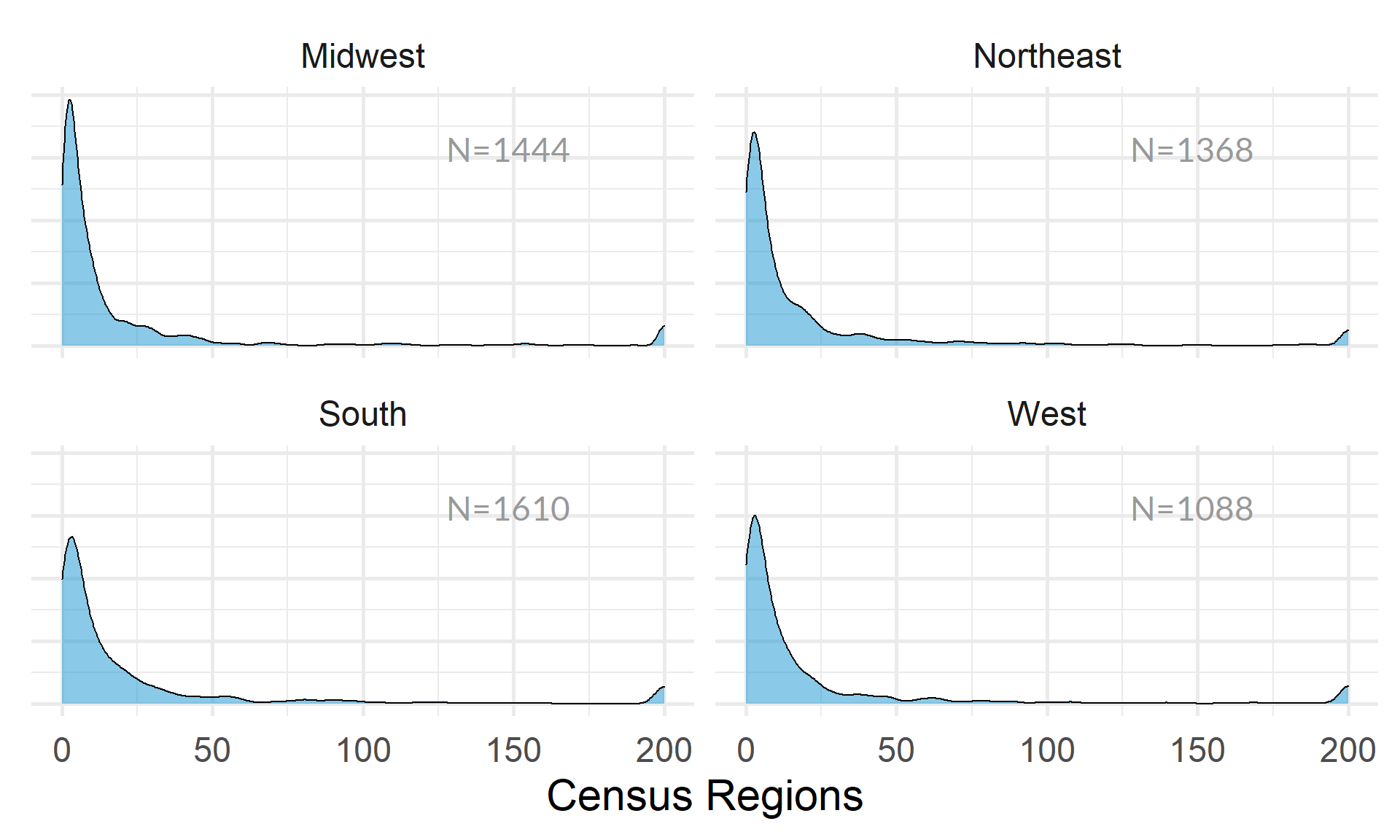

table( core2$Division ) %>% kable()

Var1	Freq
East North Central	1038
East South Central	289
Middle Atlantic	904
Mountain	303
New England	464
Pacific	785
South Atlantic	900
West North Central	406
West South Central	421

t <- table( factor(core2$Division) ) 
df <- data.frame( x=Inf, y=Inf, 
                  N=paste0( "N=", as.character(t) ), 
                  Division=names(t) )

core2 %>% 
  filter( ! is.na(Division) ) %>% 
  ggplot( aes(currentratio) )  + 
    geom_density( alpha = 0.5 ) + 
    xlab( "Census Sub-Regions (10)" ) + 
    ylab( variable.label ) +
    facet_wrap( ~ Division, nrow=3 ) + 
    theme_minimal( base_size = 22 )  + 
    theme( axis.title.y=element_blank(),
           axis.text.y=element_blank(), 
           axis.ticks.y=element_blank() ) + 
    geom_text( data=df, 
             aes(x, y, label=N ), 
             hjust=2, vjust=3, 
             color="gray60", size=6 )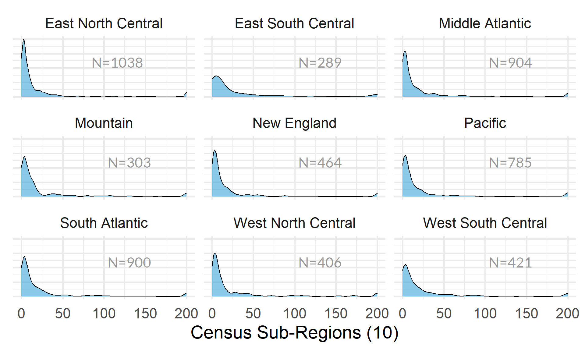 

Current Ratio by Nonprofit Size (Expenses)

ggplot( core2, aes(x = totfuncexpns )) +  
  geom_density( alpha = 0.5 ) + 
  xlim( quantile(core2$totfuncexpns, c(0.02,0.98), na.rm=T ) )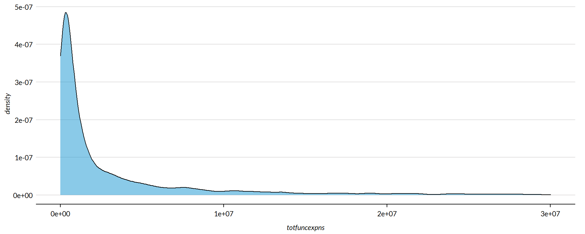

core2$totfuncexpns[ core2$totfuncexpns < 1 ] <- 1
# core2$totfuncexpns[ is.na(core2$totfuncexpns) ] <- 1

if( nrow(core2) > 10000 )
{
  core3 <- sample_n( core2, 10000 )
} else
{
  core3 <- core2
}

jplot( log10(core3$totfuncexpns), core3$currentratio, 
       xlab="Nonprofit Size (logged Expenses)", 
       ylab=variable.label,
       xaxt="n", xlim=c(3,10) )
axis( side=1, 
      at=c(3,4,5,6,7,8,9,10), 
      labels=c("1k","10k","100k","1m","10m","100m","1b","10b") )

core2 %>% 
  filter( ! is.na(exp.q) ) %>% 
  ggplot( aes(currentratio) )  + 
    geom_density( alpha = 0.5 ) + 
    labs( title="Nonprofit Size (logged expenses)" ) + 
    xlab( variable.label ) +
    facet_wrap( ~ exp.q, nrow=3 ) + 
    theme_minimal( base_size = 22 )  + 
    theme( axis.title.y=element_blank(),
           axis.text.y=element_blank(), 
           axis.ticks.y=element_blank() )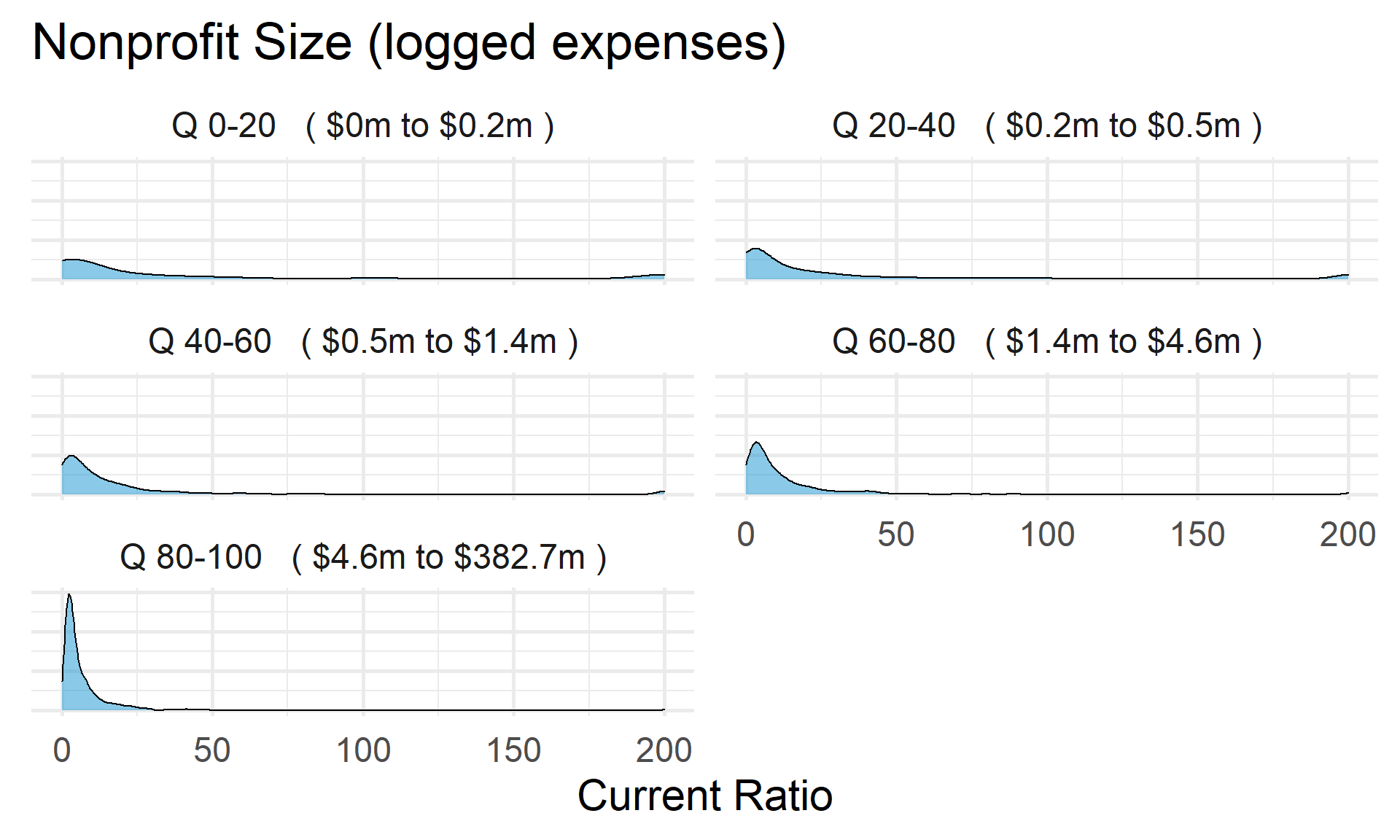

Current Ratio by Nonprofit Size (Revenue)

ggplot( core2, aes(x = totrevenue )) +  
  geom_density( alpha = 0.5 ) + 
  xlim( quantile(core2$totrevenue, c(0.02,0.98), na.rm=T ) ) + 
  theme( axis.title.y=element_blank(),
           axis.text.y=element_blank(), 
           axis.ticks.y=element_blank() )

core2$totrevenue[ core2$totrevenue < 1 ] <- 1

if( nrow(core2) > 10000 )
{
  core3 <- sample_n( core2, 10000 )
} else
{
  core3 <- core2
}

jplot( log10(core3$totrevenue), core3$currentratio, 
       xlab="Nonprofit Size (logged Revenue)", 
       ylab=variable.label,
       xaxt="n", xlim=c(3,10) )
axis( side=1, 
      at=c(3,4,5,6,7,8,9,10), 
      labels=c("1k","10k","100k","1m","10m","100m","1b","10b") )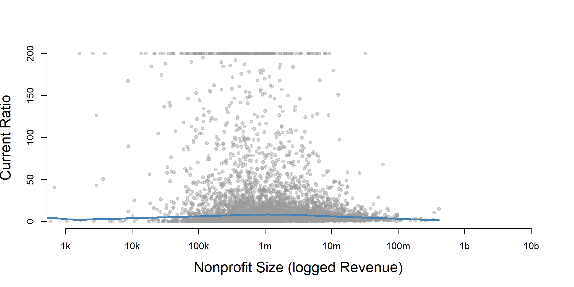

core2 %>% 
  filter( ! is.na(rev.q) ) %>% 
  ggplot( aes(currentratio) )  + 
    geom_density( alpha = 0.5 ) + 
    labs( title="Nonprofit Size (logged revenues)" ) + 
    xlab( variable.label ) +
    facet_wrap( ~ rev.q, nrow=3 ) + 
    theme_minimal( base_size = 22 )  + 
    theme( axis.title.y=element_blank(),
           axis.text.y=element_blank(), 
           axis.ticks.y=element_blank() )

Current Ratio by Nonprofit Size (Net Assets)

ggplot( core2, aes(x = totnetassetend )) +  
  geom_density( alpha = 0.5 ) + 
  xlim( quantile(core2$totnetassetend, c(0.02,0.98), na.rm=T ) ) + 
  xlab( "Net Assets" ) +
    theme( axis.title.y=element_blank(),
           axis.text.y=element_blank(), 
           axis.ticks.y=element_blank() )

core2$totnetassetend[ core2$totnetassetend < 1 ] <- NA

if( nrow(core2) > 10000 )
{
  core3 <- sample_n( core2, 10000 )
} else
{
  core3 <- core2
}

jplot( log10(core3$totnetassetend), core3$currentratio, 
       xlab="Nonprofit Size (logged Net Assets)", 
       ylab=variable.label,
       xaxt="n", xlim=c(3,10) )
axis( side=1, 
      at=c(3,4,5,6,7,8,9,10), 
      labels=c("1k","10k","100k","1m","10m","100m","1b","10b") )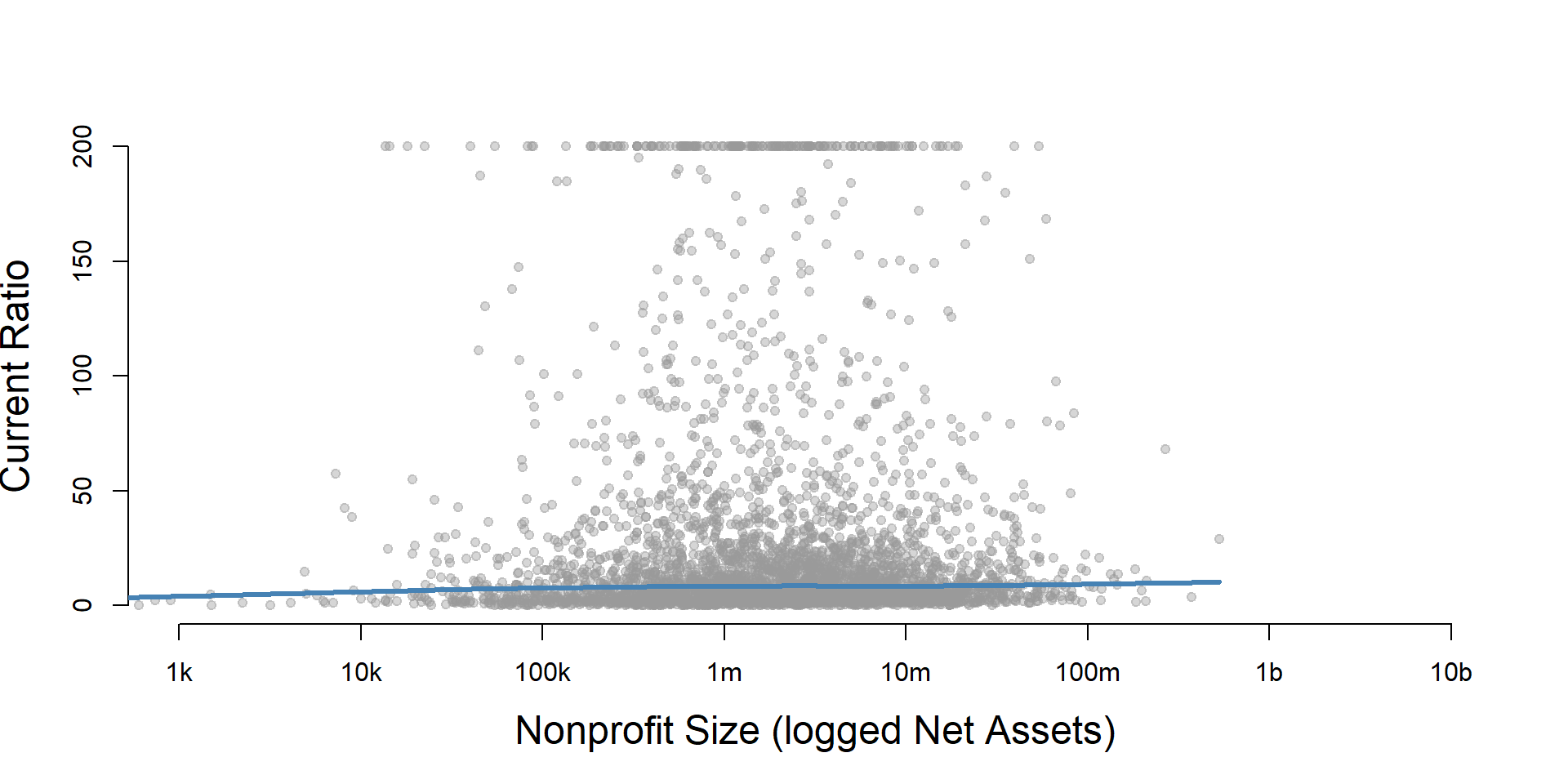

core2$totnetassetend[ core2$totnetassetend < 1 ] <- NA
core2$asset.q <- create_quantiles( var=core2$totnetassetend, n.groups=5 )

core2 %>% 
  filter( ! is.na(asset.q) ) %>% 
  ggplot( aes(currentratio) )  + 
    geom_density( alpha = 0.5 ) + 
    labs( title="Nonprofit Size (logged net assets, if assets > 0)" ) + 
    xlab( variable.label ) + 
    ylab( "" ) + 
    facet_wrap( ~ asset.q, nrow=3 ) + 
    theme_minimal( base_size = 22 )  + 
    theme( axis.title.y=element_blank(),
           axis.text.y=element_blank(), 
           axis.ticks.y=element_blank() )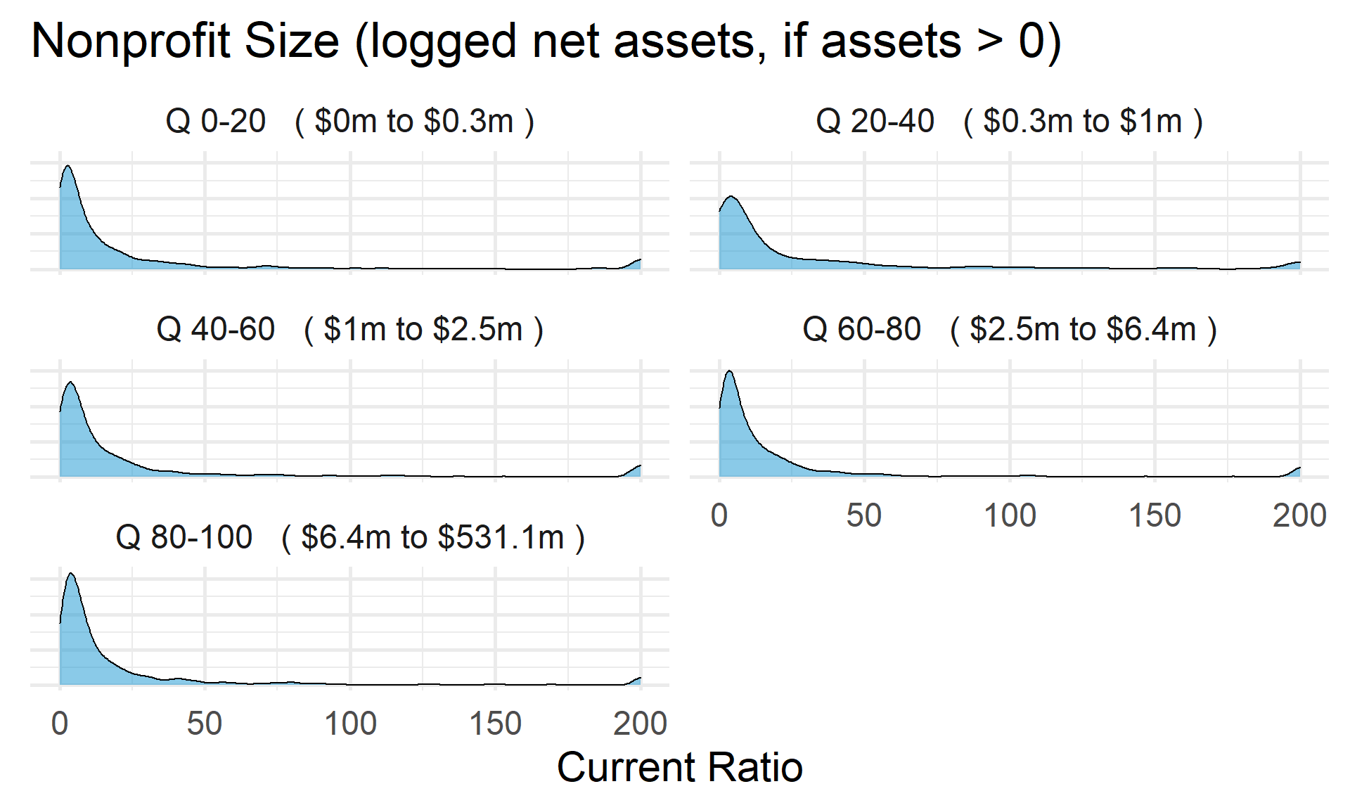

Total Assets for Comparison

core2$totassetsend[ core2$totassetsend < 1 ] <- NA
core2$tot.asset.q <- create_quantiles( var=core2$totassetsend, n.groups=5 )

if( nrow(core2) > 10000 )
{
  core3 <- sample_n( core2, 10000 )
} else
{
  core3 <- core2
}

jplot( log10(core3$totassetsend), core3$currentratio, 
       xlab="Nonprofit Size (logged Total Assets)", 
       ylab=variable.label,
       xaxt="n", xlim=c(3,10) )
axis( side=1, 
      at=c(3,4,5,6,7,8,9,10), 
      labels=c("1k","10k","100k","1m","10m","100m","1b","10b") )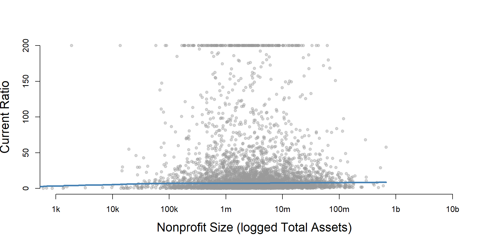

ggplot( core2, aes(x = totassetsend )) +  
  geom_density( alpha = 0.5 ) + 
  xlim( quantile(core2$totassetsend, c(0.02,0.98), na.rm=T ) ) + 
  xlab( "Net Assets" ) +
    theme( axis.title.y=element_blank(),
           axis.text.y=element_blank(), 
           axis.ticks.y=element_blank() )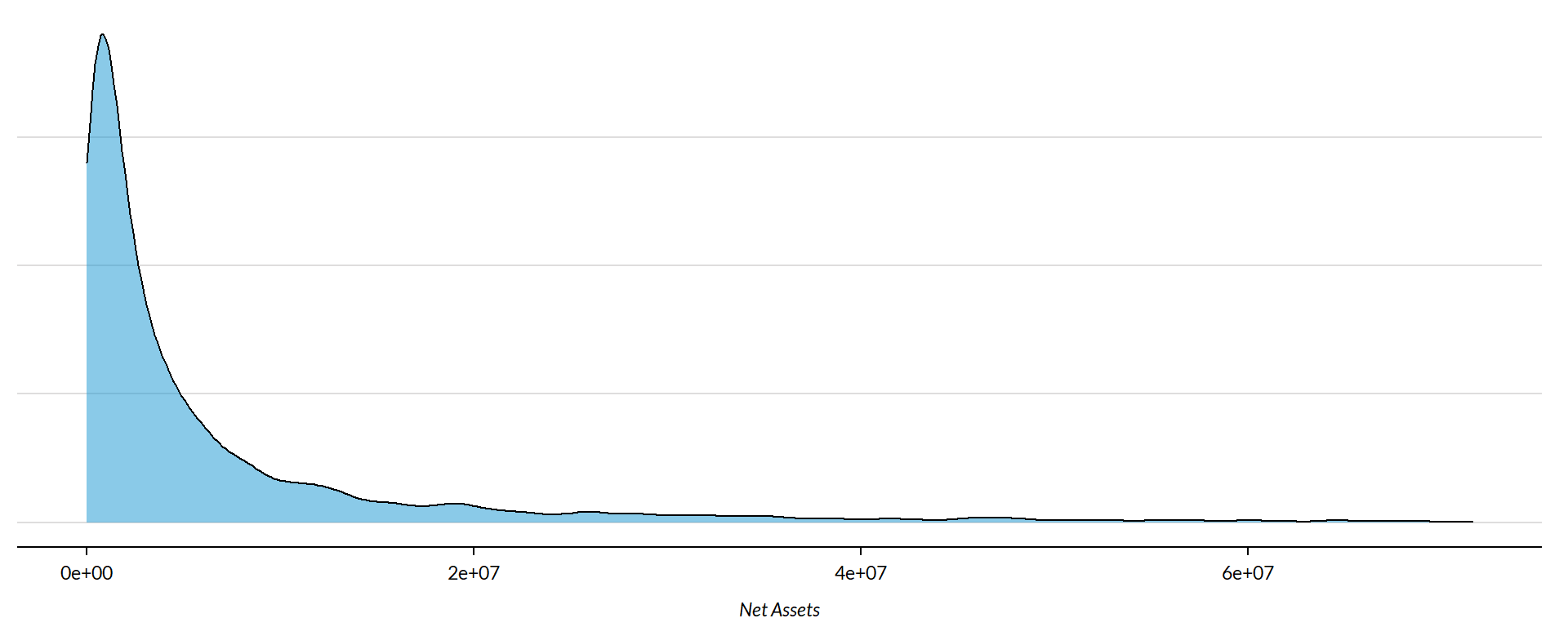

core2 %>% 
  filter( ! is.na(tot.asset.q) ) %>% 
  ggplot( aes(currentratio) )  + 
    geom_density( alpha = 0.5 ) + 
    xlab( "Nonprofit Size (logged total assets, if assets > 0)" ) + 
    ylab( variable.label ) +
    facet_wrap( ~ tot.asset.q, nrow=3 ) + 
    theme_minimal( base_size = 22 )  + 
    theme( axis.title.y=element_blank(),
           axis.text.y=element_blank(), 
           axis.ticks.y=element_blank() )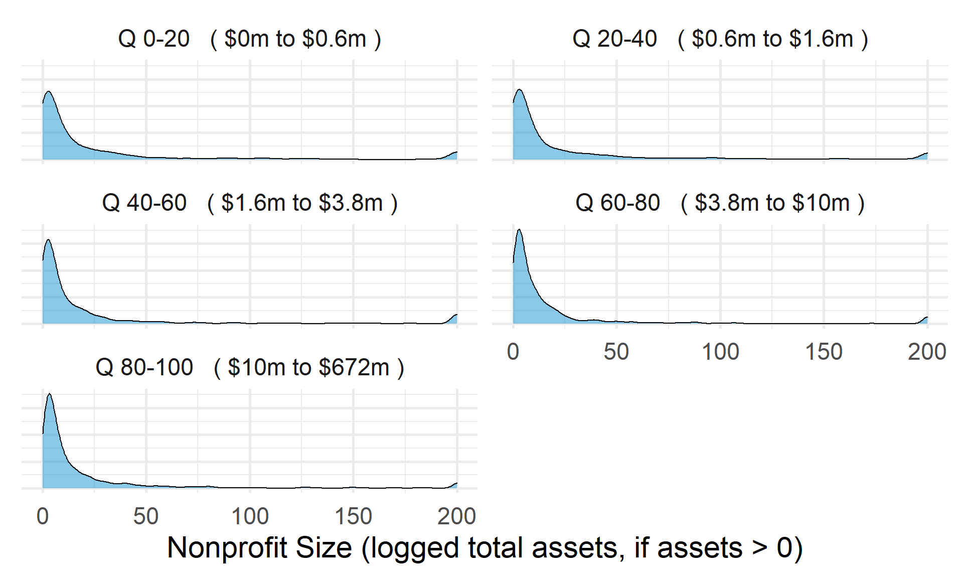

Current Ratio by Nonprofit Age

ggplot( core2, aes(x = AGE )) +  
  geom_density( alpha = 0.5 )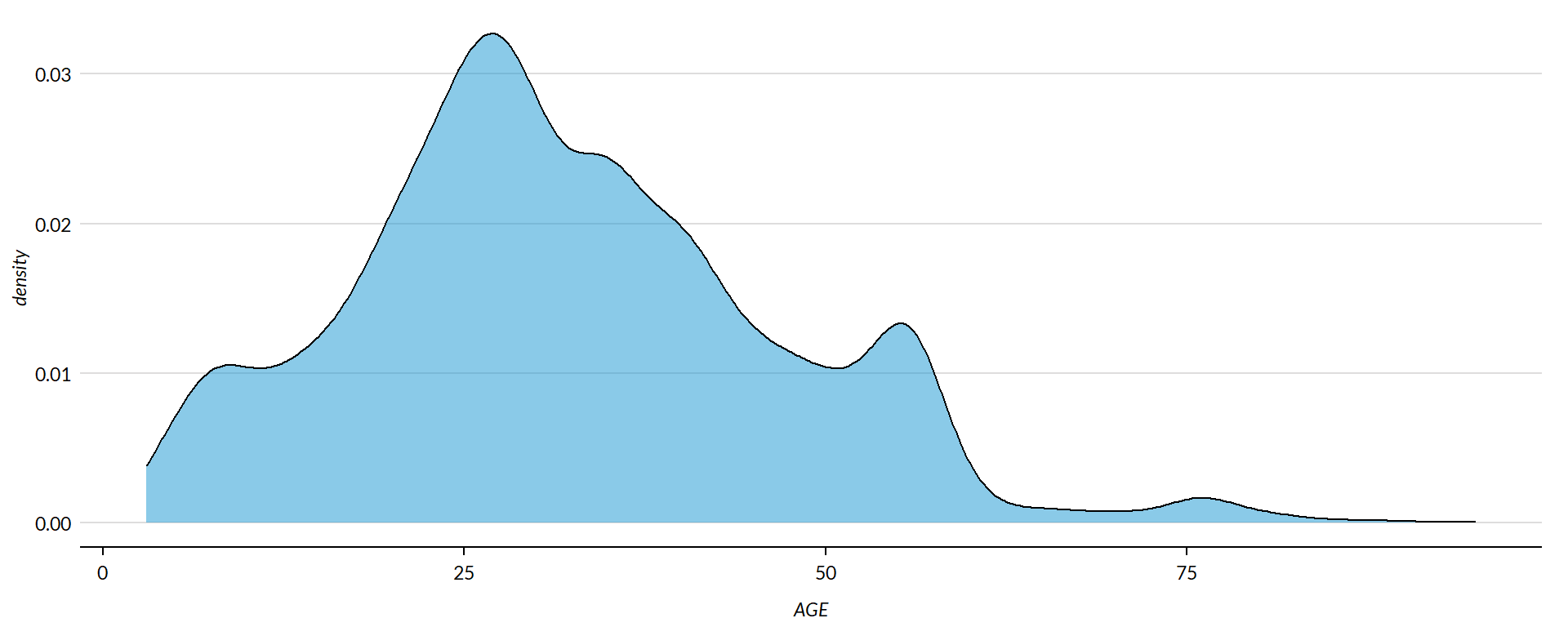  

core2$AGE[ core2$AGE < 1 ] <- NA

if( nrow(core2) > 10000 )
{
  core3 <- sample_n( core2, 10000 )
} else
{
  core3 <- core2
}

jplot( core3$AGE, core3$currentratio, 
       xlab="Nonprofit Age", 
       ylab=variable.label ) 

core2 %>% 
  filter( ! is.na(age.q) ) %>% 
  ggplot( aes(currentratio) )  + 
    geom_density( alpha = 0.5) + 
    labs( title="Nonprofit Age" ) + 
    xlab( variable.label ) +
    ylab( "" ) +
    facet_wrap( ~ age.q, nrow=3 ) + 
    theme_minimal( base_size = 22 )  + 
    theme( axis.title.y=element_blank(),
           axis.text.y=element_blank(), 
           axis.ticks.y=element_blank() )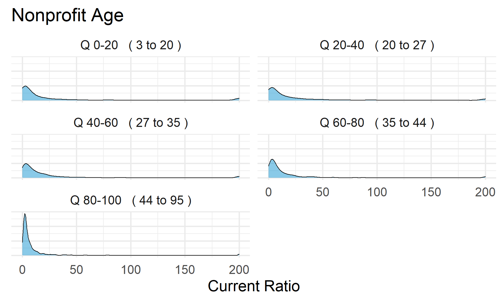

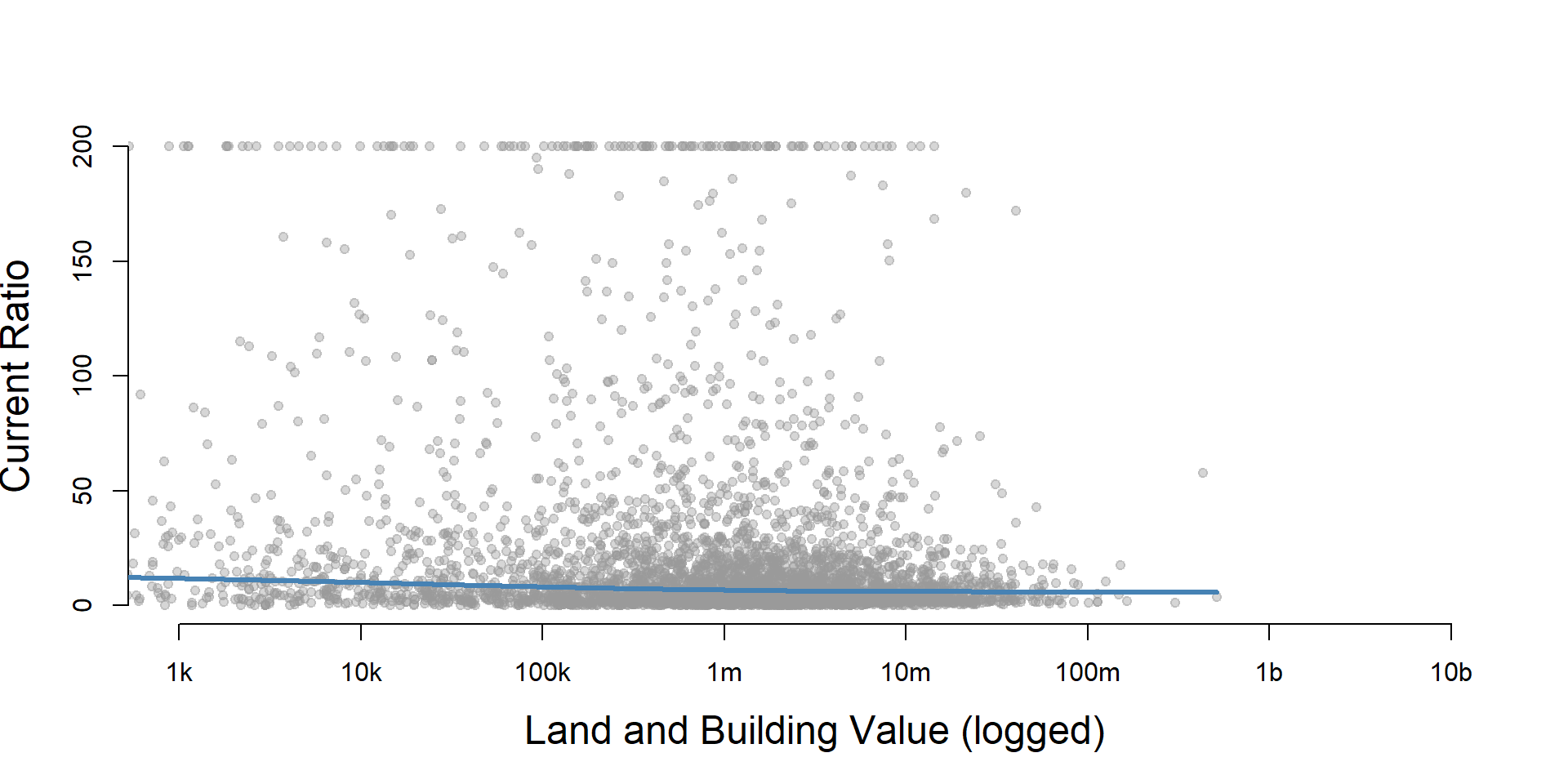
Current Ratio by Land and Building Value

ggplot( core2, aes(x = lndbldgsequipend )) +  
  geom_density( alpha = 0.5 )  

core2$lndbldgsequipend[ core2$lndbldgsequipend < 1 ] <- NA
if( nrow(core2) > 10000 )
{
  core3 <- sample_n( core2, 10000 )
} else
{
  core3 <- core2


jplot( log10(core3$lndbldgsequipend), core3$currentratio, 
       xlab="Land and Building Value (logged)", 
       ylab=variable.label,
       xaxt="n", xlim=c(3,10) )
axis( side=1, 
      at=c(3,4,5,6,7,8,9,10), 
      labels=c("1k","10k","100k","1m","10m","100m","1b","10b") )
}

core2 %>% 
  filter( ! is.na(land.q) ) %>% 
  ggplot( aes(currentratio) )  + 
    geom_density( alpha = 0.5 ) + 
    labs( title="Land and Building Value" ) + 
    xlab( variable.label ) +
    ylab( "" ) +
    facet_wrap( ~ land.q, nrow=3 ) + 
    theme_minimal( base_size = 22 )  + 
    theme( axis.title.y=element_blank(),
           axis.text.y=element_blank(), 
           axis.ticks.y=element_blank() )

Save Metrics

core.currentratio <- select( core, ein, tax_pd, currentratio )
saveRDS( core.currentratio, "03-data-ratios/m-02-current-ratio.rds" )
write.csv( core.currentratio, "03-data-ratios/m-02-current-ratio.csv" )

---

---

Metrics generated by Jesse Lecy and Nathan Dietz
Content licensed under Creative Commons: (CC BY-NC-SA 4.0)
Source code is available on GitHub

The work is supported by the
National Center for Charitable Statistics
at the Urban Institute

---