Metric 10 - Debt Management Ratio
April 8, 2022
![]()
Metric Construction
Definition & Interpretation
\[Debt\: Management \: Ratio = \frac{Total \: Liabilities}{Unrestricted \: Net \: Assets} \]
This metric measures how much an organization is relying on funding from lending entities and the amount of free, unrestricted cash it has to pay back those loans.
A high value in this metric could mean an organization is highly leveraged and thus that it has reduced ability to borrow more money in the future. Conversely, a low value indicates the organization may not be leveraging its assets to achieve the most growth and impact it could or that there is a dearth of credit available from lending entities.
Variables
Note: This data is available only for organizations that file full 990s. [Organizations with revenues <$200,000 and total assets <$500,000 have the option to not file a full 990 and file an EZ instead.]
Numerator: Total LIabilities
- On 990: Part X, line 26B
- SOI PC EXTRACTS: totliabend
- SOI PC EXTRACTS: totliabend
- On EZ: Part II, line 26B
- SOI PC EXTRACTS: totliabend
- SOI PC EXTRACTS: totliabend
- On 990: Part X, line 26B
Denominator: Unrestricted Net Assets
On 990: Part X, Line 27B -SOI PC EXTRACTS: unrstrctnetasstsend
On EZ: Not Available -SOI PC EXTRACTS: Not Available
# TEMPORARY VARIABLES
liabilities  <- ( core$totliabend)
unres_nassets <- ( core$unrstrctnetasstsend)

# can't divide by zero
unres_nassets[ unres_nassets == 0 ] <- NA

# SAVE RESULTS
core$debt_mgmnt_ratio <-  liabilities / unres_nassets

# summary( core$debt_mgmnt_ratio )
Standardize Scales
Check high and low values to see what makes sense.
x.05 <- quantile( core$debt_mgmnt_ratio, 0.05, na.rm=T )
x.95 <- quantile( core$debt_mgmnt_ratio, 0.95, na.rm=T )

ggplot( core, aes(x = debt_mgmnt_ratio ) ) +
  geom_density( alpha = 0.5) +
xlim( x.05, x.95 ) 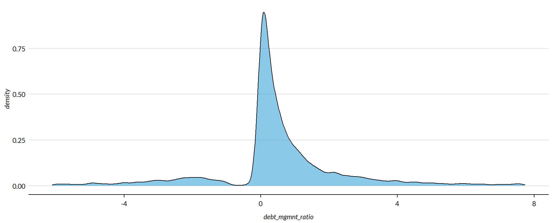
core2 <- core

# proportion of values that are negative
mean( core2$debt_mgmnt_ratio < 0, na.rm=T )
## [1] 0.1700142
core2$debt_mgmnt_ratio[ core2$debt_mgmnt_ratio < 0 ] <- 0

# proption of values above 200%
mean( core2$debt_mgmnt_ratio > 50, na.rm=T )
## [1] 0.009332522
core2$debt_mgmnt_ratio[ core2$debt_mgmnt_ratio > 50 ] <- 50


x.05 <- quantile( core$debt_mgmnt_ratio, 0.05, na.rm=T )
x.95 <- quantile( core$debt_mgmnt_ratio, 0.95, na.rm=T )

core2 <- core

# proportion of values that are negative
# mean( core2$der < 0, na.rm=T )

# proption of values above 1%
# mean( core2$der > 5, na.rm=T )

# WINSORIZATION AT 5th and 95th PERCENTILES

core2$debt_mgmnt_ratio[ core2$debt_mgmnt_ratio < x.05 ] <- x.05
core2$debt_mgmnt_ratio[ core2$debt_mgmnt_ratio > x.95 ] <- x.95
Metric Scope
Tax data is available for full 990 filers, so this metric does not describe any organizations with Gross receipts < $200,000 and Total assets < $500,000. Some organizations with receipts or assets below those thresholds may have filed a full 990, but these would be exceptions.
The data have been capped to those with values between 5% and 95% of the normal distribution to cut off outliers and exempt organizations with zero profitability (though negative values are allowed still).
Reference
Any cited works here…
Descriptive Statistics
Convert all monetary variables to thousands of dollars. Scale up metric (multiply by 100) for readability.
core2 %>%
  mutate( debt_mgmnt_ratio = debt_mgmnt_ratio * 100,
    totrevenue = totrevenue / 1000,
    totfuncexpns = totfuncexpns / 1000,
    lndbldgsequipend = lndbldgsequipend / 1000,
    totassetsend = totassetsend / 1000,
    totliabend = totliabend / 1000,
    totnetassetend = totnetassetend / 1000 ) %>%
  select( STATE,  NTEE1, NTMAJ12,
          debt_mgmnt_ratio,
          AGE,
          totrevenue, totfuncexpns,
          lndbldgsequipend, totassetsend,
          totnetassetend, totliabend ) %>%

  stargazer( type = s.type,
             digits=0,
             summary.stat = c("min","p25","median",
                              "mean","p75","max", "sd"),
             covariate.labels = c("Debt Management Ratio (x100)", "Age",
                                  "Revenue ($1k)", "Expenses($1k)",
                                  "Buildings ($1k)", "Total Assets ($1k)",
"Net Assets ($1k)", "Liabiliies ($1k)"))| Statistic | Min | Pctl(25) | Median | Mean | Pctl(75) | Max | St. Dev. |
| Debt Management Ratio (x100) | -610 | 2 | 31 | 55 | 120 | 773 | 281 |
| Age | 3 | 22 | 30 | 32 | 41 | 95 | 15 |
| Revenue (1k) | -5,377 | 259 | 909 | 4,522 | 3,672 | 408,932 | 14,286 |
| Expenses(1k) | 0 | 263 | 840 | 4,192 | 3,328 | 382,667 | 13,466 |
| Buildings (1k) | -4 | 79 | 824 | 3,504 | 2,868 | 513,509 | 13,210 |
| Total Assets (1k) | -7,552 | 778 | 2,446 | 9,262 | 7,477 | 672,021 | 27,039 |
| Net Assets (1k) | -178,870 | 156 | 1,094 | 4,553 | 4,079 | 531,068 | 15,470 |
| Liabiliies (1k) | -2,707 | 115 | 816 | 4,709 | 3,133 | 705,623 | 18,722 |
What proportion of orgs have debt management ratios equal to zero?
prop.zero <- mean( core2$debt_mgmnt_ratio == 0, na.rm=T )In the sample, 3 percent of the organizations have debt management ratios equal to zero. These organizations are dropped from subsequent graphs to keep the visualizations clean. The interpretation of the graphics should be the distributions of debt management ratios for organizations that have positive or negative values.
###
### ADD QUANTILES
###
###   function create_quantiles() defined in r-functions.R

core2$exp.q   <- create_quantiles( var=core2$totfuncexpns,   n.groups=5 )
core2$rev.q   <- create_quantiles( var=core2$totrevenue,     n.groups=5 )
core2$asset.q <- create_quantiles( var=core2$totnetassetend, n.groups=5 )
core2$age.q   <- create_quantiles( var=core2$AGE,            n.groups=5 )
core2$land.q   <- create_quantiles( var=core2$lndbldgsequipend,    n.groups=5 )
Debt Management Ratio Density
min.x <- min( core2$debt_mgmnt_ratio, na.rm=T )
max.x <- max( core2$debt_mgmnt_ratio, na.rm=T )

ggplot( core2, aes(x = debt_mgmnt_ratio )) +
  geom_density( alpha = 0.5 ) +
  xlim( min.x, max.x  ) +
  xlab( variable.label ) +
  theme( axis.title.y=element_blank(),
         axis.text.y=element_blank(),
         axis.ticks.y=element_blank() )
Debt Management Ratio by NTEE Major Code
core3 <- core2 %>% filter( ! is.na(NTEE1) )
table( core3$NTEE1) %>% sort(decreasing=TRUE) %>% kable()| Var1 | Freq |
|---|---|
| Housing | 2837 |
| Community Development | 1585 |
| Human Services | 1102 |
t <- table( factor(core3$NTEE1) )
df <- data.frame( x=Inf, y=Inf,
                  N=paste0( "N=", as.character(t) ),
                  NTEE1=names(t) )

ggplot( core3, aes( x=debt_mgmnt_ratio ) ) +
  geom_density( alpha = 0.5) +
  # xlim( -0.1, 1 ) +
  labs( title="Nonprofit Subsectors" ) +
  xlab( variable.label ) +
  facet_wrap( ~ NTEE1, nrow=1 ) +
    theme_minimal( base_size = 15 )  +
    theme( axis.title.y=element_blank(),
           axis.text.y=element_blank(),
           axis.ticks.y=element_blank(),
           strip.text = element_text( face="bold") ) +  # size=20
  geom_text( data=df,
             aes(x, y, label=N ),
             hjust=2, vjust=3,
             color="gray60", size=6 )
Debt Management Ratio by Region
table( core2$Region) %>% kable()| Var1 | Freq |
|---|---|
| Midwest | 1444 |
| Northeast | 1368 |
| South | 1610 |
| West | 1088 |
t <- table( factor(core2$Region) )
df <- data.frame( x=Inf, y=Inf,
                  N=paste0( "N=", as.character(t) ),
                  Region=names(t) )

core2 %>%
  filter( ! is.na(Region) ) %>%
  ggplot( aes(debt_mgmnt_ratio) )  +
    geom_density( alpha = 0.5 ) +
    xlab( "Census Regions" ) +
    ylab( variable.label ) +
    facet_wrap( ~ Region, nrow=3 ) +
    theme_minimal( base_size = 22 )  +
    theme( axis.title.y=element_blank(),
           axis.text.y=element_blank(),
           axis.ticks.y=element_blank() ) +
    geom_text( data=df,
             aes(x, y, label=N ),
             hjust=2, vjust=3,
             color="gray60", size=6 )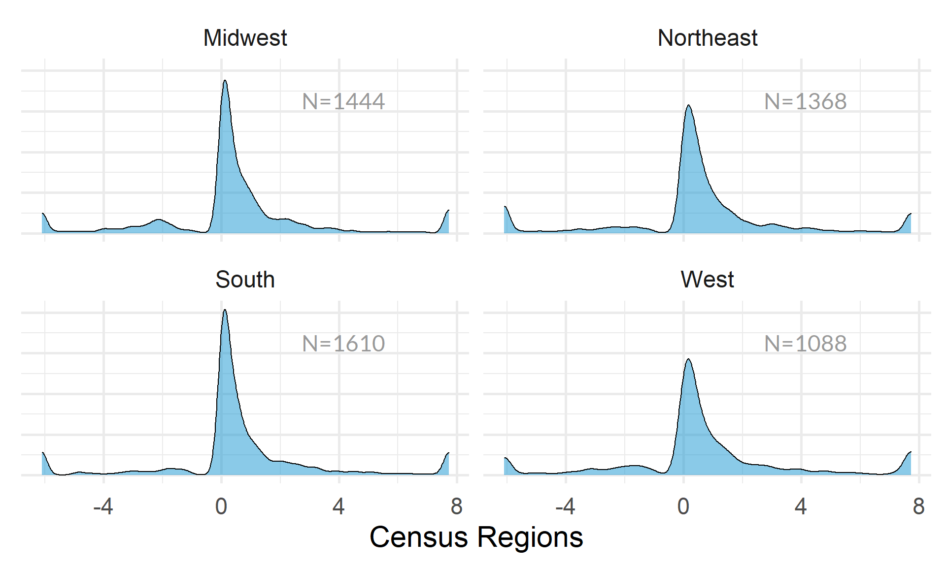
table( core2$Division ) %>% kable()| Var1 | Freq |
|---|---|
| East North Central | 1038 |
| East South Central | 289 |
| Middle Atlantic | 904 |
| Mountain | 303 |
| New England | 464 |
| Pacific | 785 |
| South Atlantic | 900 |
| West North Central | 406 |
| West South Central | 421 |
t <- table( factor(core2$Division) )
df <- data.frame( x=Inf, y=Inf,
                  N=paste0( "N=", as.character(t) ),
                  Division=names(t) )

core2 %>%
  filter( ! is.na(Division) ) %>%
  ggplot( aes(debt_mgmnt_ratio) )  +
    geom_density( alpha = 0.5 ) +
    xlab( "Census Sub-Regions (10)" ) +
    ylab( variable.label ) +
    facet_wrap( ~ Division, nrow=3 ) +
    theme_minimal( base_size = 22 )  +
    theme( axis.title.y=element_blank(),
           axis.text.y=element_blank(),
           axis.ticks.y=element_blank() ) +
    geom_text( data=df,
             aes(x, y, label=N ),
             hjust=2, vjust=3,
color="gray60", size=6 ) 
Debt Management Ratio by Nonprofit Size (Expenses)
ggplot( core2, aes(x = totfuncexpns )) +
  geom_density( alpha = 0.5 ) +
  xlim( quantile(core2$totfuncexpns, c(0.02,0.98), na.rm=T ) )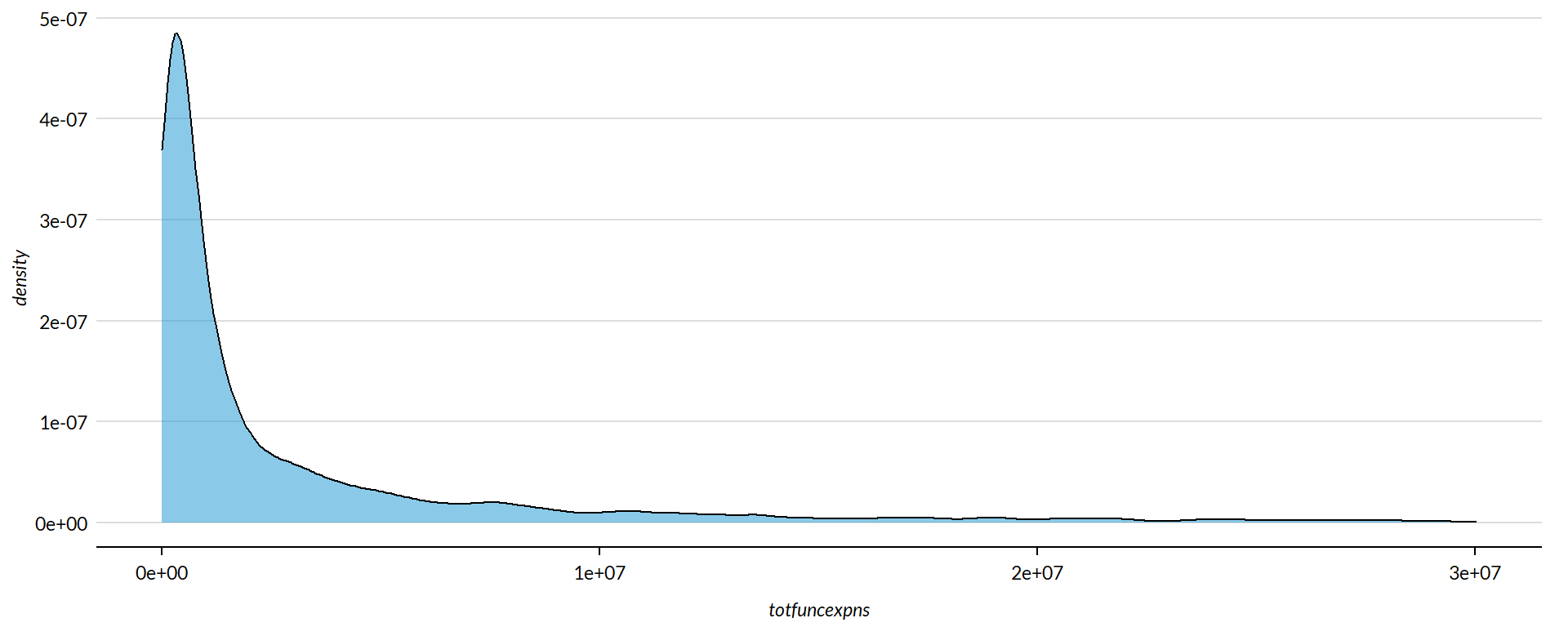
core2$totfuncexpns[ core2$totfuncexpns < 1 ] <- 1
# core2$totfuncexpns[ is.na(core2$totfuncexpns) ] <- 1

if( nrow(core2) > 10000 )
{
  core3 <- sample_n( core2, 10000 )
} else
{
  core3 <- core2
}

jplot( log10(core3$totfuncexpns), core3$debt_mgmnt_ratio,
       xlab="Nonprofit Size (logged Expenses)",
       ylab=variable.label,
       xaxt="n", xlim=c(3,10) )
axis( side=1,
      at=c(3,4,5,6,7,8,9,10),
      labels=c("1k","10k","100k","1m","10m","100m","1b","10b") )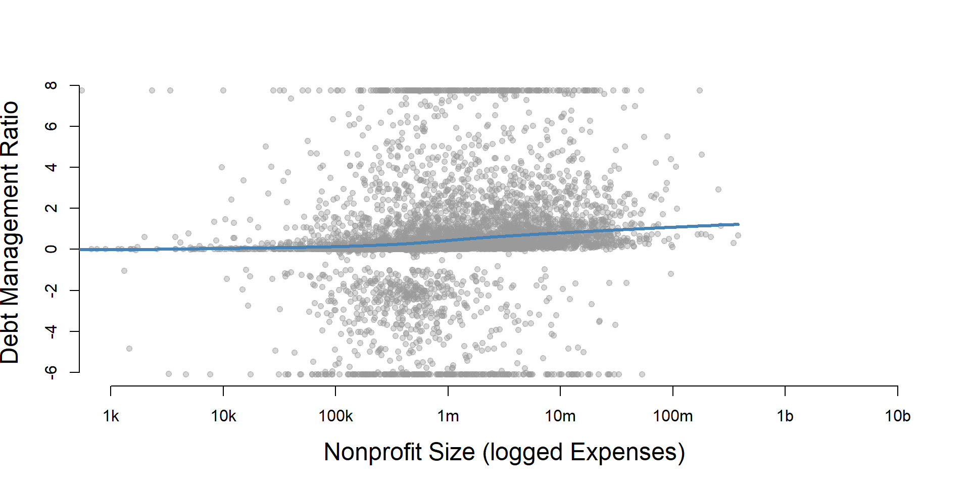
core2 %>%
  filter( ! is.na(exp.q) ) %>%
  ggplot( aes(debt_mgmnt_ratio) )  +
    geom_density( alpha = 0.5) +
    labs( title="Nonprofit Size (logged expenses)" ) +
    xlab( variable.label ) +
    facet_wrap( ~ exp.q, nrow=3 ) +
    theme_minimal( base_size = 22 )  +
    theme( axis.title.y=element_blank(),
           axis.text.y=element_blank(),
           axis.ticks.y=element_blank() )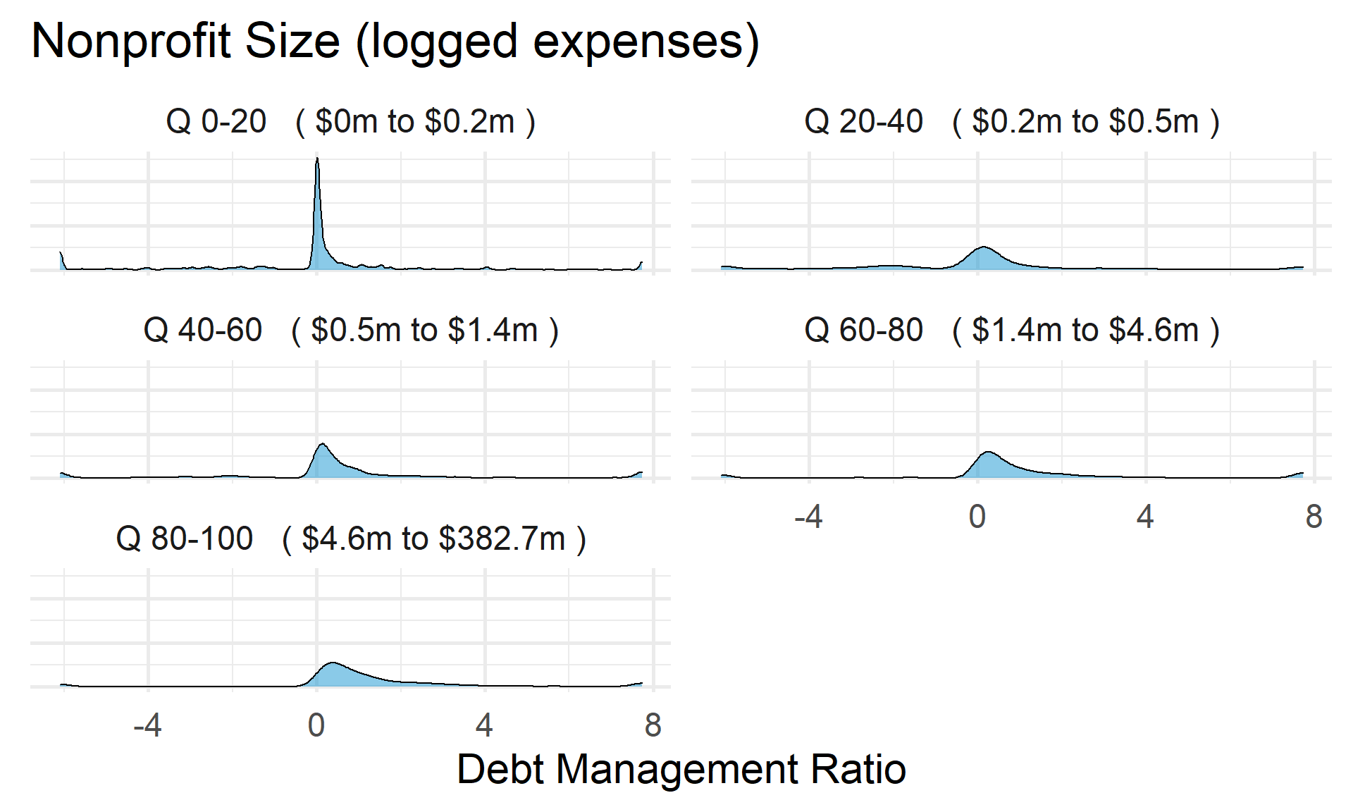
Debt Management Ratio by Nonprofit Size (Revenue)
ggplot( core2, aes(x = totrevenue )) +
  geom_density( alpha = 0.5 ) +
  xlim( quantile(core2$totrevenue, c(0.02,0.98), na.rm=T ) ) +
  theme( axis.title.y=element_blank(),
           axis.text.y=element_blank(),
           axis.ticks.y=element_blank() )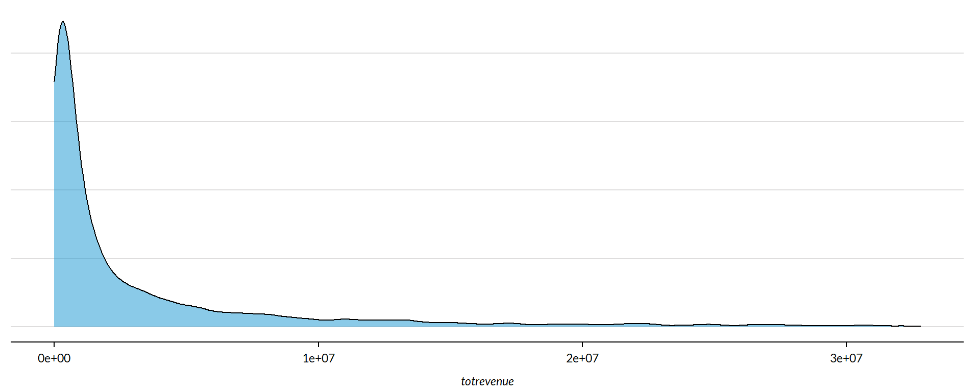
core2$totrevenue[ core2$totrevenue < 1 ] <- 1

if( nrow(core2) > 10000 )
{
  core3 <- sample_n( core2, 10000 )
} else
{
  core3 <- core2
}

jplot( log10(core3$totrevenue), core3$debt_mgmnt_ratio,
       xlab="Nonprofit Size (logged Revenue)",
       ylab=variable.label,
       xaxt="n", xlim=c(3,10) )
axis( side=1,
      at=c(3,4,5,6,7,8,9,10),
      labels=c("1k","10k","100k","1m","10m","100m","1b","10b") )
core2 %>%
  filter( ! is.na(rev.q) ) %>%
  ggplot( aes(debt_mgmnt_ratio) )  +
    geom_density( alpha = 0.5 ) +
    labs( title="Nonprofit Size (logged revenues)" ) +
    xlab( variable.label ) +
    facet_wrap( ~ rev.q, nrow=3 ) +
    theme_minimal( base_size = 22 )  +
    theme( axis.title.y=element_blank(),
           axis.text.y=element_blank(),
           axis.ticks.y=element_blank() )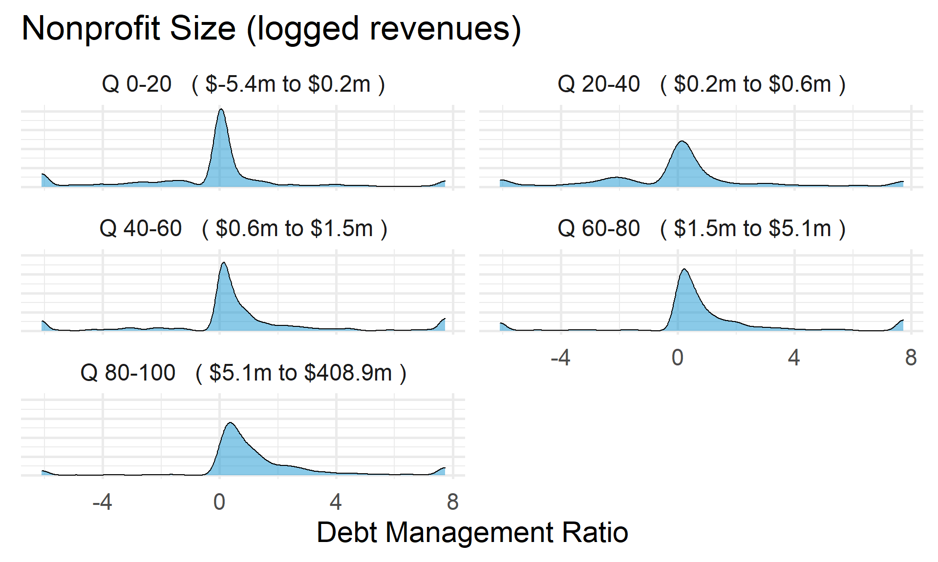
Debt Management Ratio by Nonprofit Size (Net Assets)
ggplot( core2, aes(x = totnetassetend )) +
  geom_density( alpha = 0.5) +
  xlim( quantile(core2$totnetassetend, c(0.02,0.98), na.rm=T ) ) +
  xlab( "Net Assets" ) +
    theme( axis.title.y=element_blank(),
           axis.text.y=element_blank(),
           axis.ticks.y=element_blank() )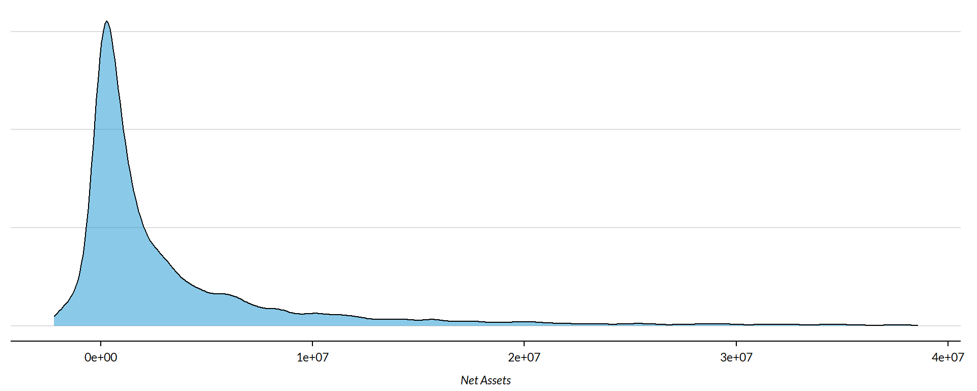
core2$totnetassetend[ core2$totnetassetend < 1 ] <- NA

if( nrow(core2) > 10000 )
{
  core3 <- sample_n( core2, 10000 )
} else
{
  core3 <- core2
}

jplot( log10(core3$totnetassetend), core3$debt_mgmnt_ratio,
       xlab="Nonprofit Size (logged Net Assets)",
       ylab=variable.label,
       xaxt="n", xlim=c(3,10) )
axis( side=1,
      at=c(3,4,5,6,7,8,9,10),
      labels=c("1k","10k","100k","1m","10m","100m","1b","10b") )
core2$totnetassetend[ core2$totnetassetend < 1 ] <- NA
core2$asset.q <- create_quantiles( var=core2$totnetassetend, n.groups=5 )

core2 %>%
  filter( ! is.na(asset.q) ) %>%
  ggplot( aes(debt_mgmnt_ratio) )  +
    geom_density( alpha = 0.5 ) +
    labs( title="Nonprofit Size (logged net assets, if assets > 0)" ) +
    xlab( variable.label ) +
    ylab( "" ) +
    facet_wrap( ~ asset.q, nrow=3 ) +
    theme_minimal( base_size = 22 )  +
    theme( axis.title.y=element_blank(),
           axis.text.y=element_blank(),
           axis.ticks.y=element_blank() )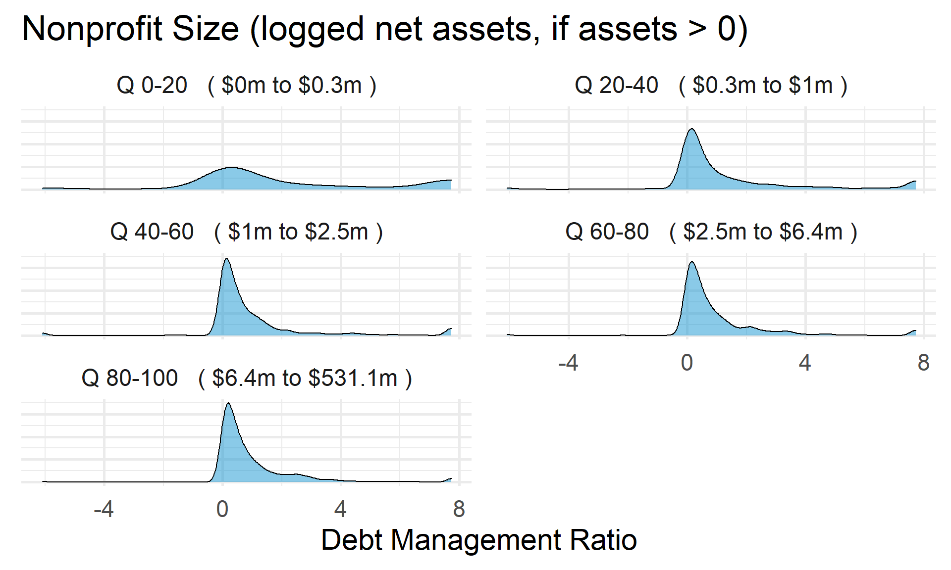
Total Assets for Comparison
core2$totassetsend[ core2$totassetsend < 1 ] <- NA
core2$tot.asset.q <- create_quantiles( var=core2$totassetsend, n.groups=5 )

if( nrow(core2) > 10000 )
{
  core3 <- sample_n( core2, 10000 )
} else
{
  core3 <- core2
}

jplot( log10(core3$totassetsend), core3$debt_mgmnt_ratio,
       xlab="Nonprofit Size (logged Total Assets)",
       ylab=variable.label,
       xaxt="n", xlim=c(3,10) )
axis( side=1,
      at=c(3,4,5,6,7,8,9,10),
      labels=c("1k","10k","100k","1m","10m","100m","1b","10b") )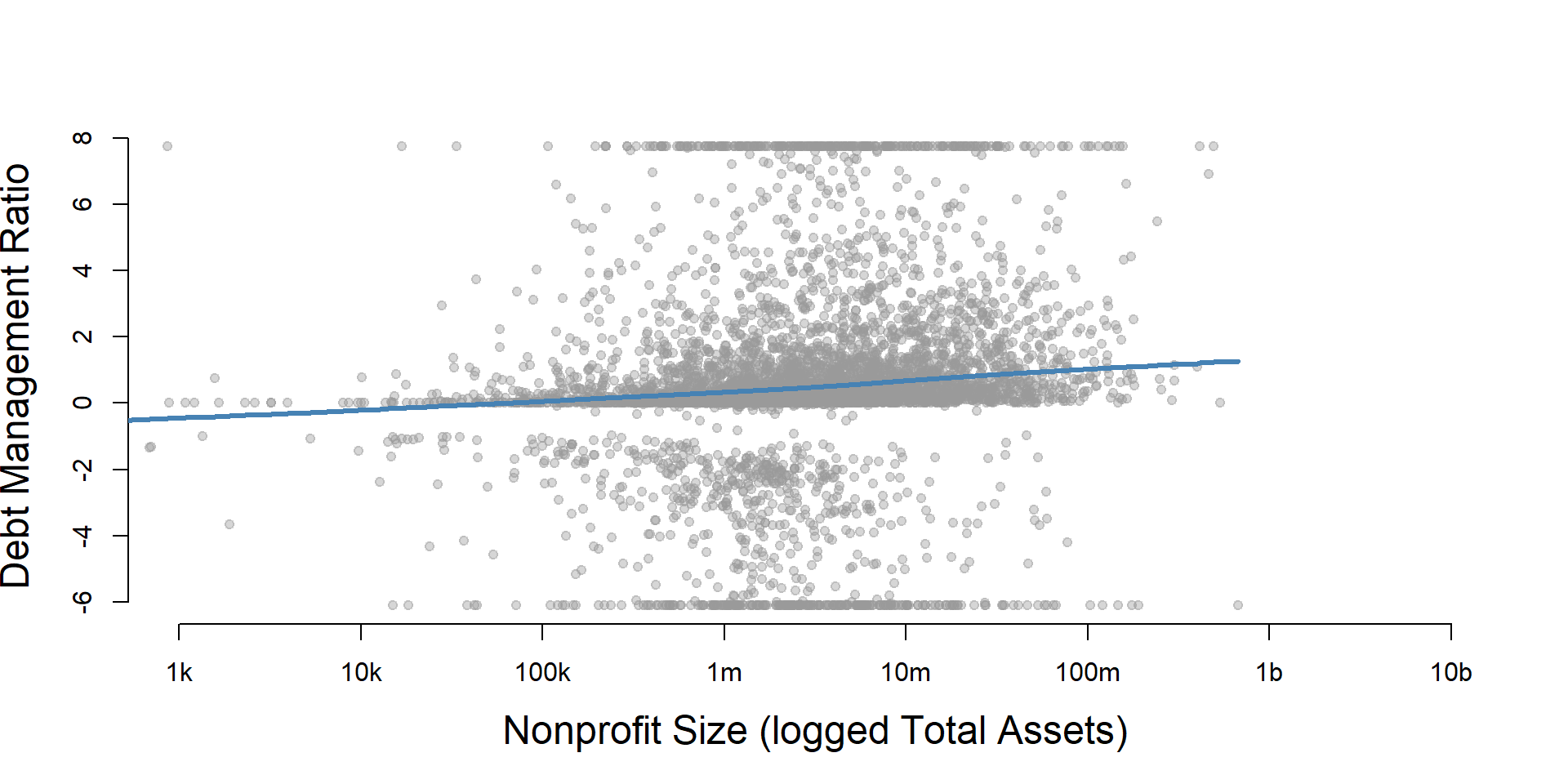
ggplot( core2, aes(x = totassetsend )) +
  geom_density( alpha = 0.5) +
  xlim( quantile(core2$totassetsend, c(0.02,0.98), na.rm=T ) ) +
  xlab( "Net Assets" ) +
    theme( axis.title.y=element_blank(),
           axis.text.y=element_blank(),
           axis.ticks.y=element_blank() )
core2 %>%
  filter( ! is.na(tot.asset.q) ) %>%
  ggplot( aes(debt_mgmnt_ratio) )  +
    geom_density( alpha = 0.5 ) +
    xlab( "Nonprofit Size (logged total assets, if assets > 0)" ) +
    ylab( variable.label ) +
    facet_wrap( ~ tot.asset.q, nrow=3 ) +
    theme_minimal( base_size = 22 )  +
    theme( axis.title.y=element_blank(),
           axis.text.y=element_blank(),
           axis.ticks.y=element_blank() )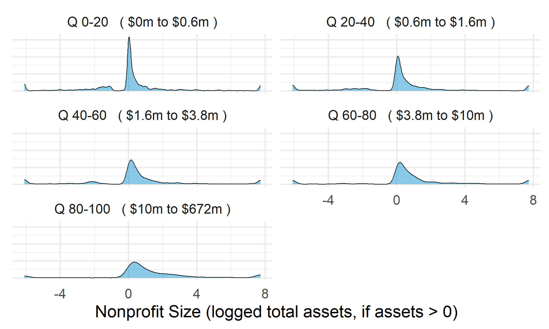
Debt Management Ratio by Nonprofit Age
ggplot( core2, aes(x = AGE )) +
geom_density( alpha = 0.5 ) 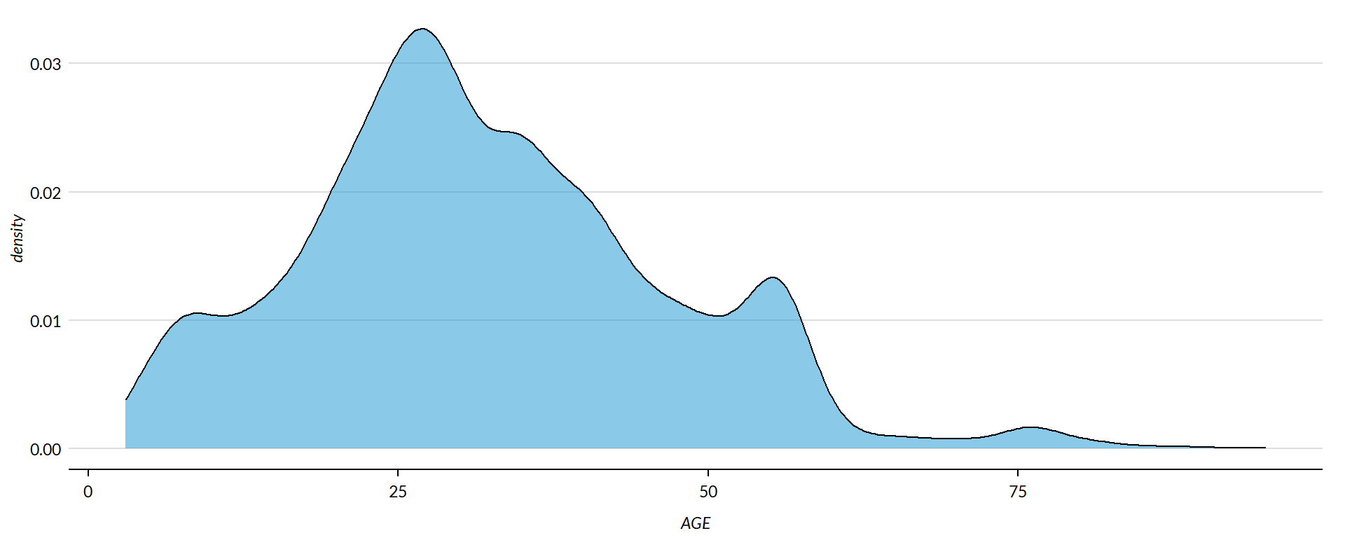
core2$AGE[ core2$AGE < 1 ] <- NA

if( nrow(core2) > 10000 )
{
  core3 <- sample_n( core2, 10000 )
} else
{
  core3 <- core2
}

jplot( core3$AGE, core3$debt_mgmnt_ratio,
       xlab="Nonprofit Age",
ylab=variable.label ) 
core2 %>%
  filter( ! is.na(age.q) ) %>%
  ggplot( aes(debt_mgmnt_ratio) )  +
    geom_density( alpha = 0.5 ) +
    labs( title="Nonprofit Age" ) +
    xlab( variable.label ) +
    ylab( "" ) +
    facet_wrap( ~ age.q, nrow=3 ) +
    theme_minimal( base_size = 22 )  +
    theme( axis.title.y=element_blank(),
           axis.text.y=element_blank(),
           axis.ticks.y=element_blank() )
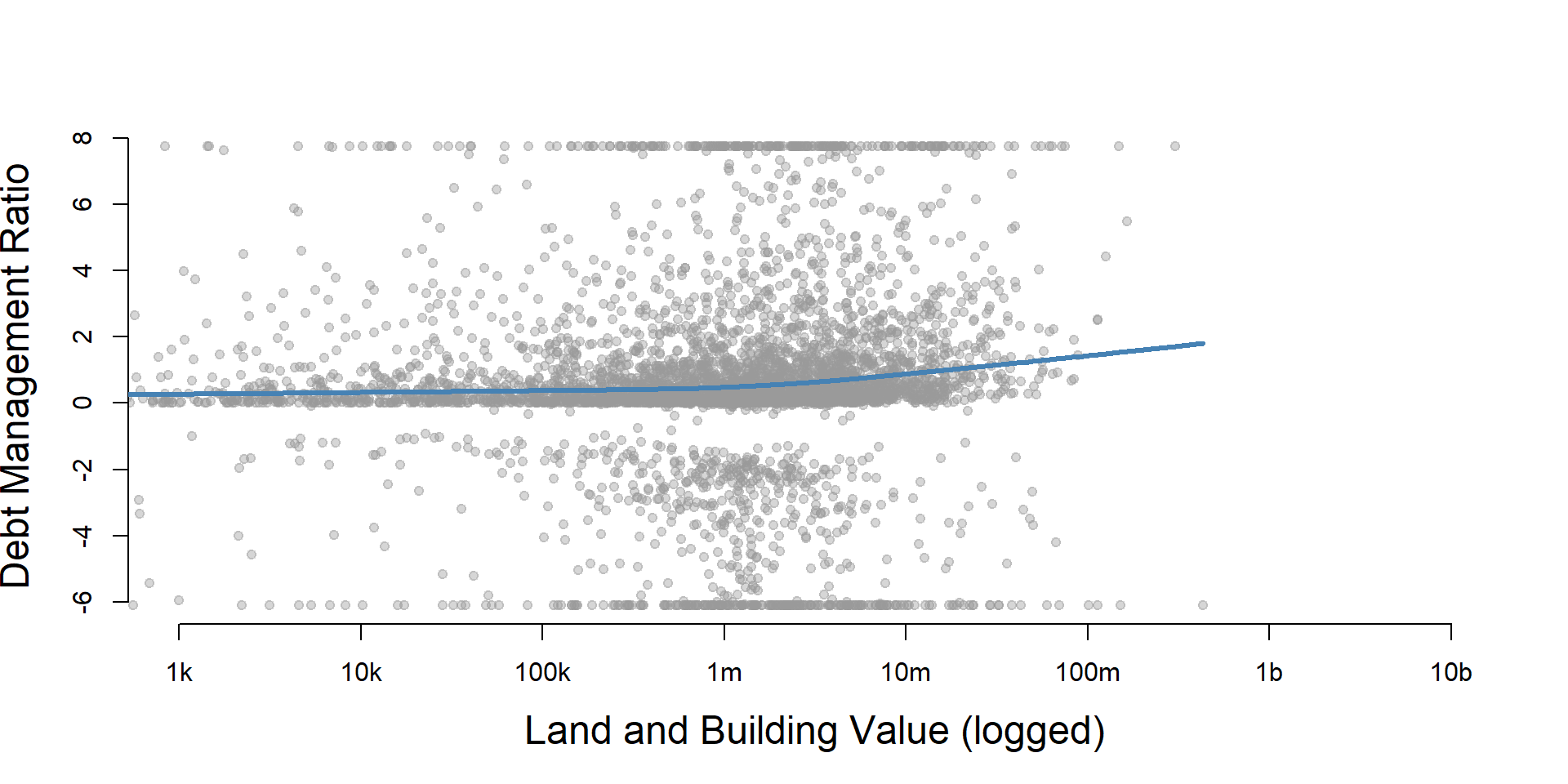
Debt Management Ratio by Land and Building Value
ggplot( core2, aes(x = lndbldgsequipend )) +
geom_density( alpha = 0.5 ) 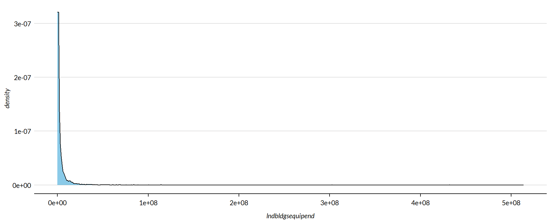
core2$lndbldgsequipend[ core2$lndbldgsequipend < 1 ] <- NA
if( nrow(core2) > 10000 )
{
  core3 <- sample_n( core2, 10000 )
} else
{
  core3 <- core2


jplot( log10(core3$lndbldgsequipend), core3$debt_mgmnt_ratio,
       xlab="Land and Building Value (logged)",
       ylab=variable.label,
       xaxt="n", xlim=c(3,10) )
axis( side=1,
      at=c(3,4,5,6,7,8,9,10),
      labels=c("1k","10k","100k","1m","10m","100m","1b","10b") )
}
core2 %>%
  filter( ! is.na(land.q) ) %>%
  ggplot( aes(debt_mgmnt_ratio) )  +
    geom_density( alpha = 0.5 ) +
    labs( title="Land and Building Value" ) +
    xlab( variable.label ) +
    ylab( "" ) +
    facet_wrap( ~ land.q, nrow=3 ) +
    theme_minimal( base_size = 22 )  +
    theme( axis.title.y=element_blank(),
           axis.text.y=element_blank(),
           axis.ticks.y=element_blank() )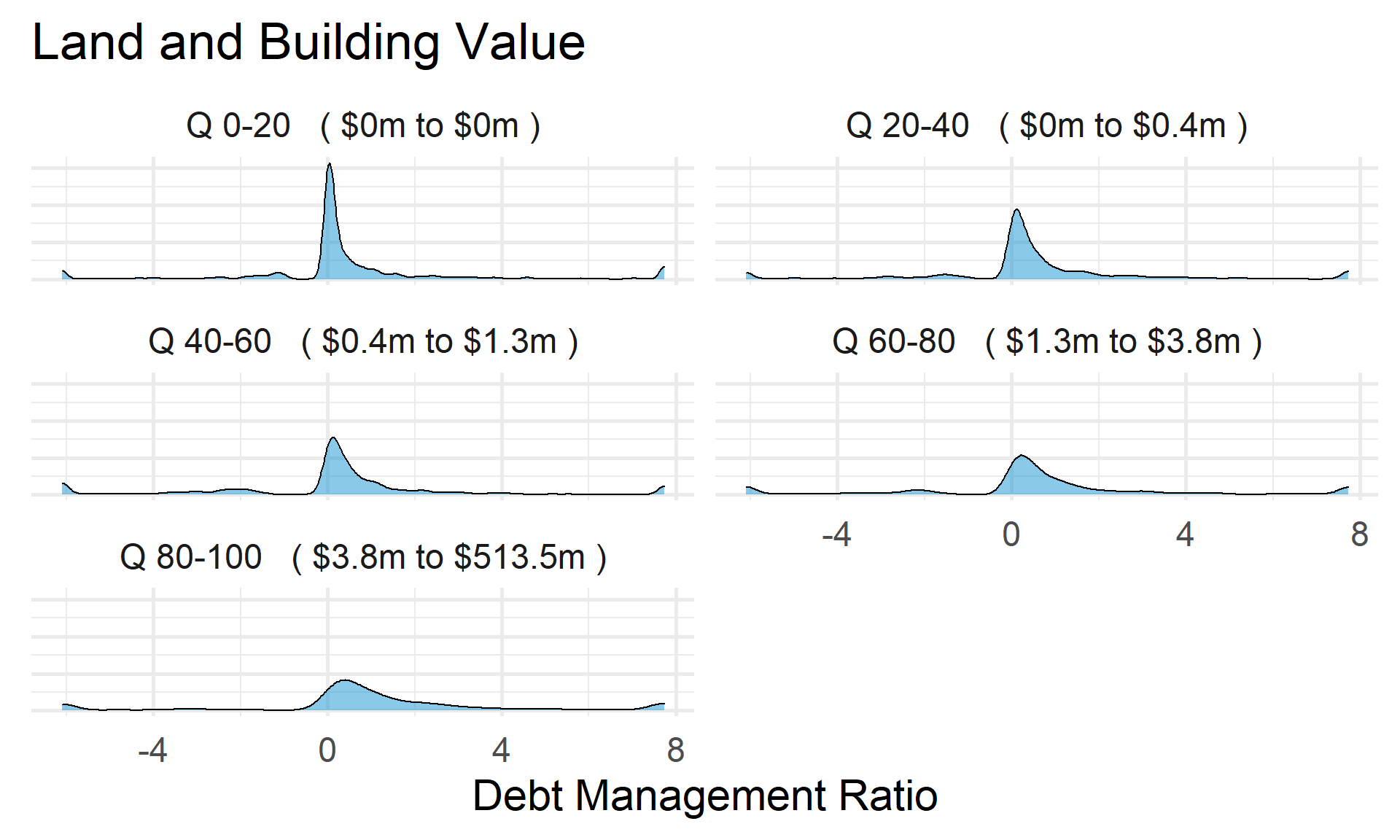
Save Metrics
core.debt_mgmnt_ratio <- select( core, ein, tax_pd, debt_mgmnt_ratio )
saveRDS( core.debt_mgmnt_ratio, "03-data-ratios/m-10-debt-management-ratio.rds" )
write.csv( core.debt_mgmnt_ratio, "03-data-ratios/m-10-debt-management-ratio.csv" )