Metric 12- Quick Ratio
April 8, 2022
![]()
Metric Construction
Definition & Interpretation
\[Quick\:Ratio = \frac{Cash + Short \text-term \: Investments + Current\: Receivables}{Current \: Liabilities} \]
This metric indicates how well an organization can cover its liabilities with its readily available cash. When an organization has a quick ratio of 1, its quick assets are equal to its current liabilities. This also indicates that the organization can pay off its current debts without selling its long-term assets. If an organization has a quick ratio higher than 1, this means that it owns more quick assets than current liabilities.
Variables
Note: This data is available only for organizations that file full 990s. [Organizations with revenues <$200,000 and total assets <$500,000 have the option to not file a full 990 and file an EZ instead.]
Numerator: Quick Assets [or cash + short-term investments + current receivables]
- On 990: (Part X, line 1B) + (Part X, line 2B) + (Part X, line 3B) +
(Part X, line 4B)
- SOI PC EXTRACTS:
(nonintcashend+svngstempinvend+pldgegrntrcvblend+accntsrcvblend)
- SOI PC EXTRACTS:
(nonintcashend+svngstempinvend+pldgegrntrcvblend+accntsrcvblend)
- On EZ: Part I, line 22 [cash and short-term investments only]
- SOI PC EXTRACTS: Not Available
- SOI PC EXTRACTS: Not Available
- On 990: (Part X, line 1B) + (Part X, line 2B) + (Part X, line 3B) +
(Part X, line 4B)
Denominator: (Accounts payable + grants payable)
On 990: (Part X, line 17B) + (Part X, line 18B) -SOI PC EXTRACTS: accntspayableend+grntspayableend
On EZ: Not Available -SOI PC EXTRACTS: Not Available
# TEMPORARY VARIABLES
quick_assets  <- (core$nonintcashend+core$svngstempinvend+core$pldgegrntrcvblend+core$accntsrcvblend)
payables <- ( core$accntspayableend+core$grntspayableend)

# can't divide by zero
payables[ payables == 0 ] <- NA

# SAVE RESULTS
core$quick_ratio <-  quick_assets / payables

# summary( core$quick_ratio )
Standardize Scales
Check high and low values to see what makes sense.
x.05 <- quantile( core$quick_ratio, 0.05, na.rm=T )
x.95 <- quantile( core$quick_ratio, 0.95, na.rm=T )

ggplot( core, aes(x = quick_ratio ) ) +
  geom_density( alpha = 0.5) +
xlim( x.05, x.95 ) 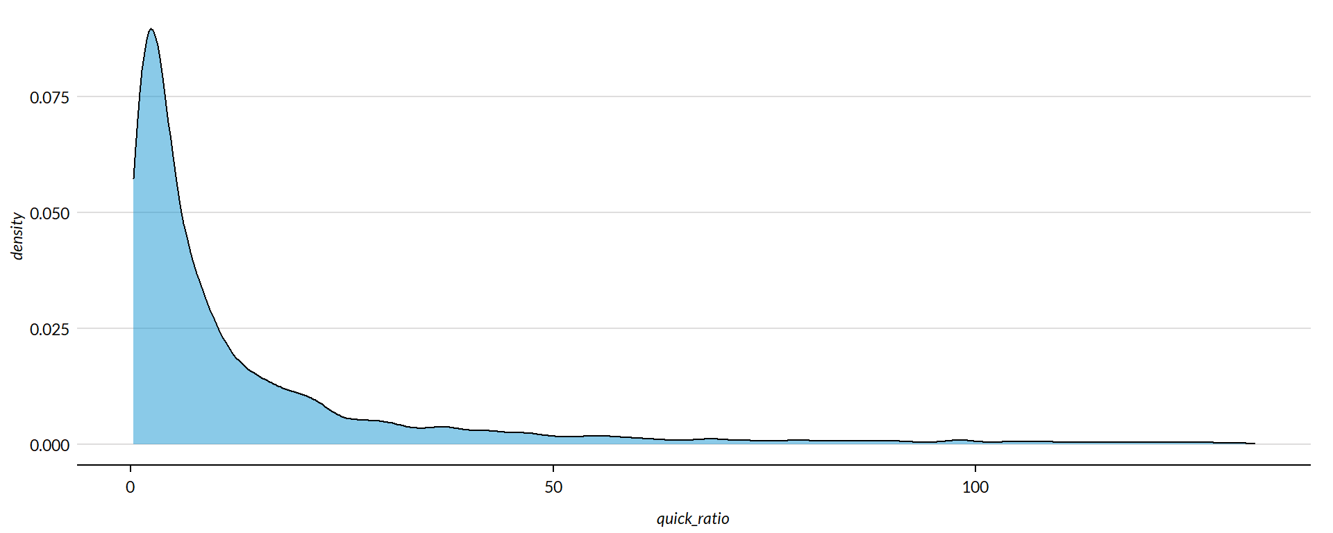
core2 <- core

# proportion of values that are negative
mean( core2$quick_ratio < 0, na.rm=T )
## [1] 0.003170577
core2$quick_ratio[ core2$quick_ratio < 0 ] <- 0

# proption of values above 200%
mean( core2$quick_ratio > 50, na.rm=T )
## [1] 0.1056859
core2$quick_ratio[ core2$quick_ratio > 50 ] <- 50


x.05 <- quantile( core$quick_ratio, 0.05, na.rm=T )
x.95 <- quantile( core$quick_ratio, 0.95, na.rm=T )

core2 <- core

# proportion of values that are negative
# mean( core2$der < 0, na.rm=T )

# proption of values above 1%
# mean( core2$der > 5, na.rm=T )

# WINSORIZATION AT 5th and 95th PERCENTILES

core2$quick_ratio[ core2$quick_ratio < x.05 ] <- x.05
core2$quick_ratio[ core2$quick_ratio > x.95 ] <- x.95
Metric Scope
Tax data is available for full 990 filers, so this metric does not describe any organizations with Gross receipts < $200,000 and Total assets < $500,000. Some organizations with receipts or assets below those thresholds may have filed a full 990, but these would be exceptions.
The data have been capped to those with values between 5% and 95% of the normal distribution to cut off outliers and exempt organizations with zero profitability (though negative values are allowed still).
Reference
Any cited works here…
Descriptive Statistics
Note: All monetary variables have been converted to thousands of dollars.
core2 %>%
  mutate( # quick_ratio = quick_ratio * 10000,
    totrevenue = totrevenue / 1000,
    totfuncexpns = totfuncexpns / 1000,
    lndbldgsequipend = lndbldgsequipend / 1000,
    totassetsend = totassetsend / 1000,
    totliabend = totliabend / 1000,
    totnetassetend = totnetassetend / 1000) %>%
  select( STATE,  NTEE1, NTMAJ12,
          quick_ratio,
          AGE,
          totrevenue, totfuncexpns,
          lndbldgsequipend, totassetsend,
          totnetassetend, totliabend ) %>%

  stargazer( type = s.type,
             digits=2,
             summary.stat = c("min","p25","median",
                              "mean","p75","max", "sd"),
             covariate.labels = c("Quick Ratio", "Age",
                                  "Revenue ($1k)", "Expenses($1k)",
                                  "Buildings ($1k)", "Total Assets ($1k)",
"Net Assets ($1k)", "Liabiliies ($1k)"))| Statistic | Min | Pctl(25) | Median | Mean | Pctl(75) | Max | St. Dev. |
| Quick Ratio | 0.30 | 2.10 | 5.73 | 19.01 | 17.36 | 133.02 | 32.81 |
| Age | 3 | 22 | 30 | 32.04 | 41 | 95 | 14.75 |
| Revenue (1k) | -5,376.77 | 258.90 | 909.40 | 4,521.71 | 3,672.25 | 408,932.00 | 14,285.64 |
| Expenses(1k) | 0.00 | 263.50 | 840.06 | 4,192.08 | 3,327.50 | 382,666.50 | 13,465.77 |
| Buildings (1k) | -4.48 | 79.14 | 824.25 | 3,504.47 | 2,868.50 | 513,508.80 | 13,210.06 |
| Total Assets (1k) | -7,552.11 | 777.90 | 2,446.11 | 9,261.85 | 7,477.25 | 672,021.00 | 27,038.89 |
| Net Assets (1k) | -178,869.70 | 155.67 | 1,093.86 | 4,553.27 | 4,078.70 | 531,067.70 | 15,470.31 |
| Liabiliies (1k) | -2,707.10 | 115.44 | 815.58 | 4,708.51 | 3,133.16 | 705,623.10 | 18,721.86 |
What proportion of orgs have quick ratios equal to zero?
prop.zero <- mean( core2$quick_ratio == 0, na.rm=T )In the sample, 0 percent of the organizations have quick ratios equal to zero, meaning they have no quick cash available. These organizations are dropped from subsequent graphs to keep the visualizations clean. The interpretation of the graphics should be the distributions of quick ratios for organizations that have positive or negative values.
###
### ADD QUANTILES
###
###   function create_quantiles() defined in r-functions.R

core2$exp.q   <- create_quantiles( var=core2$totfuncexpns,   n.groups=5 )
core2$rev.q   <- create_quantiles( var=core2$totrevenue,     n.groups=5 )
core2$asset.q <- create_quantiles( var=core2$totnetassetend, n.groups=5 )
core2$age.q   <- create_quantiles( var=core2$AGE,            n.groups=5 )
core2$land.q <- create_quantiles (var=core2$lndbldgsequipend,n.groups=5 )
Quick Ratio Density
min.x <- min( core2$quick_ratio, na.rm=T )
max.x <- max( core2$quick_ratio, na.rm=T )

ggplot( core2, aes(x = quick_ratio )) +
  geom_density( alpha = 0.5 ) +
  xlim( min.x, max.x  ) +
  xlab( variable.label ) +
  theme( axis.title.y=element_blank(),
         axis.text.y=element_blank(),
         axis.ticks.y=element_blank() )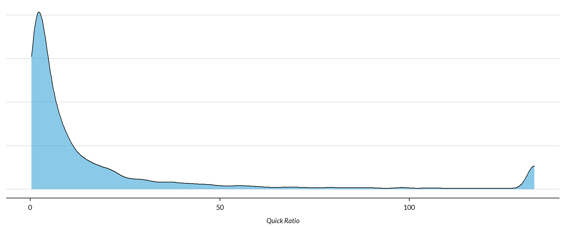
Quick Ratio by NTEE Major Code
core3 <- core2 %>% filter( ! is.na(NTEE1) )
table( core3$NTEE1) %>% sort(decreasing=TRUE) %>% kable()| Var1 | Freq |
|---|---|
| Housing | 2837 |
| Community Development | 1585 |
| Human Services | 1102 |
t <- table( factor(core3$NTEE1) )
df <- data.frame( x=Inf, y=Inf,
                  N=paste0( "N=", as.character(t) ),
                  NTEE1=names(t) )

ggplot( core3, aes( x=quick_ratio ) ) +
  geom_density( alpha = 0.5) +
  # xlim( -0.1, 1 ) +
  labs( title="Nonprofit Subsectors" ) +
  xlab( variable.label ) +
  facet_wrap( ~ NTEE1, nrow=1 ) +
    theme_minimal( base_size = 15 )  +
    theme( axis.title.y=element_blank(),
           axis.text.y=element_blank(),
           axis.ticks.y=element_blank(),
           strip.text = element_text( face="bold") ) +  # size=20
  geom_text( data=df,
             aes(x, y, label=N ),
             hjust=2, vjust=3,
             color="gray60", size=6 )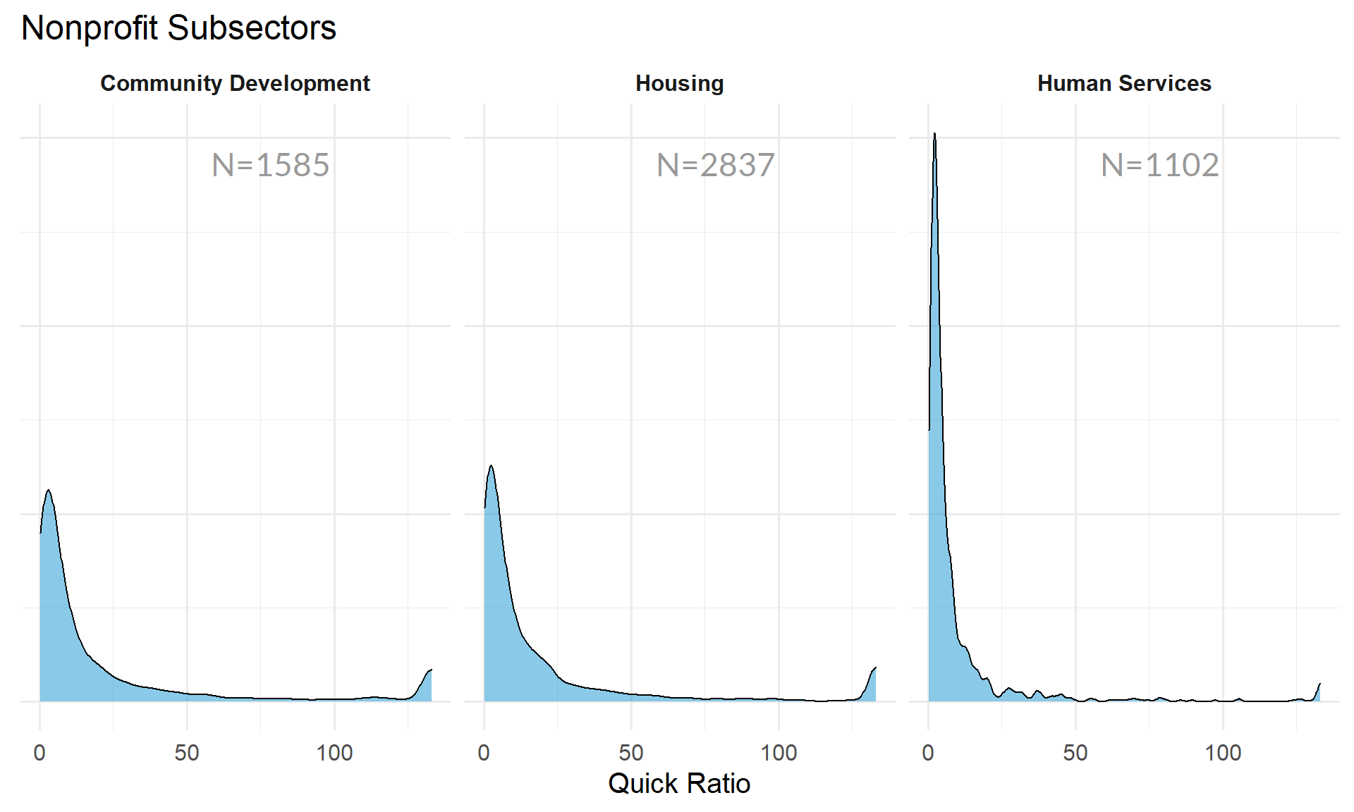
Quick Ratio by Region
table( core2$Region) %>% kable()| Var1 | Freq |
|---|---|
| Midwest | 1444 |
| Northeast | 1368 |
| South | 1610 |
| West | 1088 |
t <- table( factor(core2$Region) )
df <- data.frame( x=Inf, y=Inf,
                  N=paste0( "N=", as.character(t) ),
                  Region=names(t) )

core2 %>%
  filter( ! is.na(Region) ) %>%
  ggplot( aes(quick_ratio) )  +
    geom_density( alpha = 0.5 ) +
    xlab( "Census Regions" ) +
    ylab( variable.label ) +
    facet_wrap( ~ Region, nrow=3 ) +
    theme_minimal( base_size = 22 )  +
    theme( axis.title.y=element_blank(),
           axis.text.y=element_blank(),
           axis.ticks.y=element_blank() ) +
    geom_text( data=df,
             aes(x, y, label=N ),
             hjust=2, vjust=3,
             color="gray60", size=6 )
table( core2$Division ) %>% kable()| Var1 | Freq |
|---|---|
| East North Central | 1038 |
| East South Central | 289 |
| Middle Atlantic | 904 |
| Mountain | 303 |
| New England | 464 |
| Pacific | 785 |
| South Atlantic | 900 |
| West North Central | 406 |
| West South Central | 421 |
t <- table( factor(core2$Division) )
df <- data.frame( x=Inf, y=Inf,
                  N=paste0( "N=", as.character(t) ),
                  Division=names(t) )

core2 %>%
  filter( ! is.na(Division) ) %>%
  ggplot( aes(quick_ratio) )  +
    geom_density( alpha = 0.5 ) +
    xlab( "Census Sub-Regions (10)" ) +
    ylab( variable.label ) +
    facet_wrap( ~ Division, nrow=3 ) +
    theme_minimal( base_size = 22 )  +
    theme( axis.title.y=element_blank(),
           axis.text.y=element_blank(),
           axis.ticks.y=element_blank() ) +
    geom_text( data=df,
             aes(x, y, label=N ),
             hjust=2, vjust=3,
color="gray60", size=6 ) 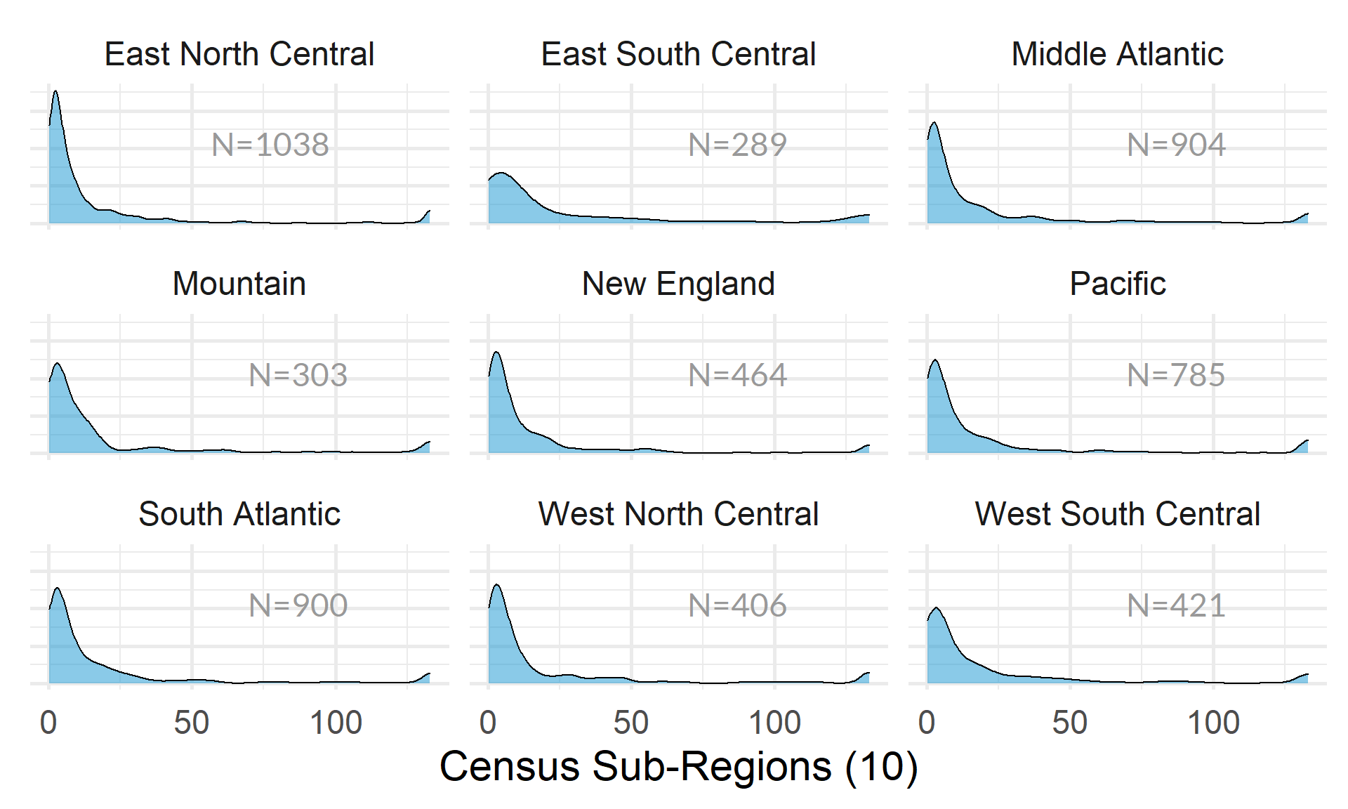
Quick Ratio by Nonprofit Size (Expenses)
ggplot( core2, aes(x = totfuncexpns )) +
  geom_density( alpha = 0.5 ) +
  xlim( quantile(core2$totfuncexpns, c(0.02,0.98), na.rm=T ) )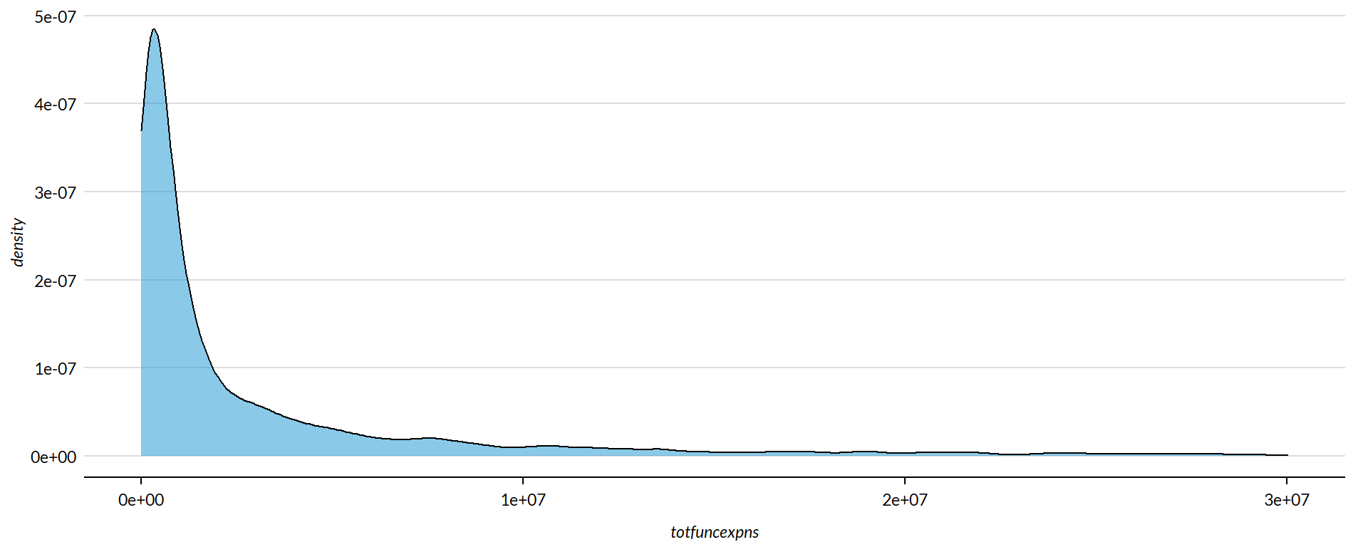
core2$totfuncexpns[ core2$totfuncexpns < 1 ] <- 1
# core2$totfuncexpns[ is.na(core2$totfuncexpns) ] <- 1

if( nrow(core2) > 10000 )
{
  core3 <- sample_n( core2, 10000 )
} else
{
  core3 <- core2
}

jplot( log10(core3$totfuncexpns), core3$quick_ratio,
       xlab="Nonprofit Size (logged Expenses)",
       ylab=variable.label,
       xaxt="n", xlim=c(3,10) )
axis( side=1,
      at=c(3,4,5,6,7,8,9,10),
      labels=c("1k","10k","100k","1m","10m","100m","1b","10b") )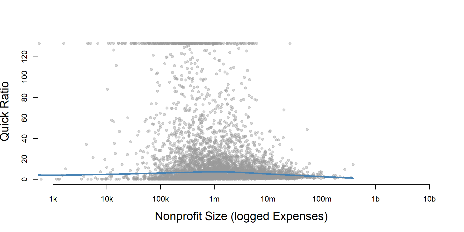
core2 %>%
  filter( ! is.na(exp.q) ) %>%
  ggplot( aes(quick_ratio) )  +
    geom_density( alpha = 0.5) +
    labs( title="Nonprofit Size (logged expenses)" ) +
    xlab( variable.label ) +
    facet_wrap( ~ exp.q, nrow=3 ) +
    theme_minimal( base_size = 22 )  +
    theme( axis.title.y=element_blank(),
           axis.text.y=element_blank(),
           axis.ticks.y=element_blank() )
Quick Ratio by Nonprofit Size (Revenue)
ggplot( core2, aes(x = totrevenue )) +
  geom_density( alpha = 0.5 ) +
  xlim( quantile(core2$totrevenue, c(0.02,0.98), na.rm=T ) ) +
  theme( axis.title.y=element_blank(),
           axis.text.y=element_blank(),
           axis.ticks.y=element_blank() )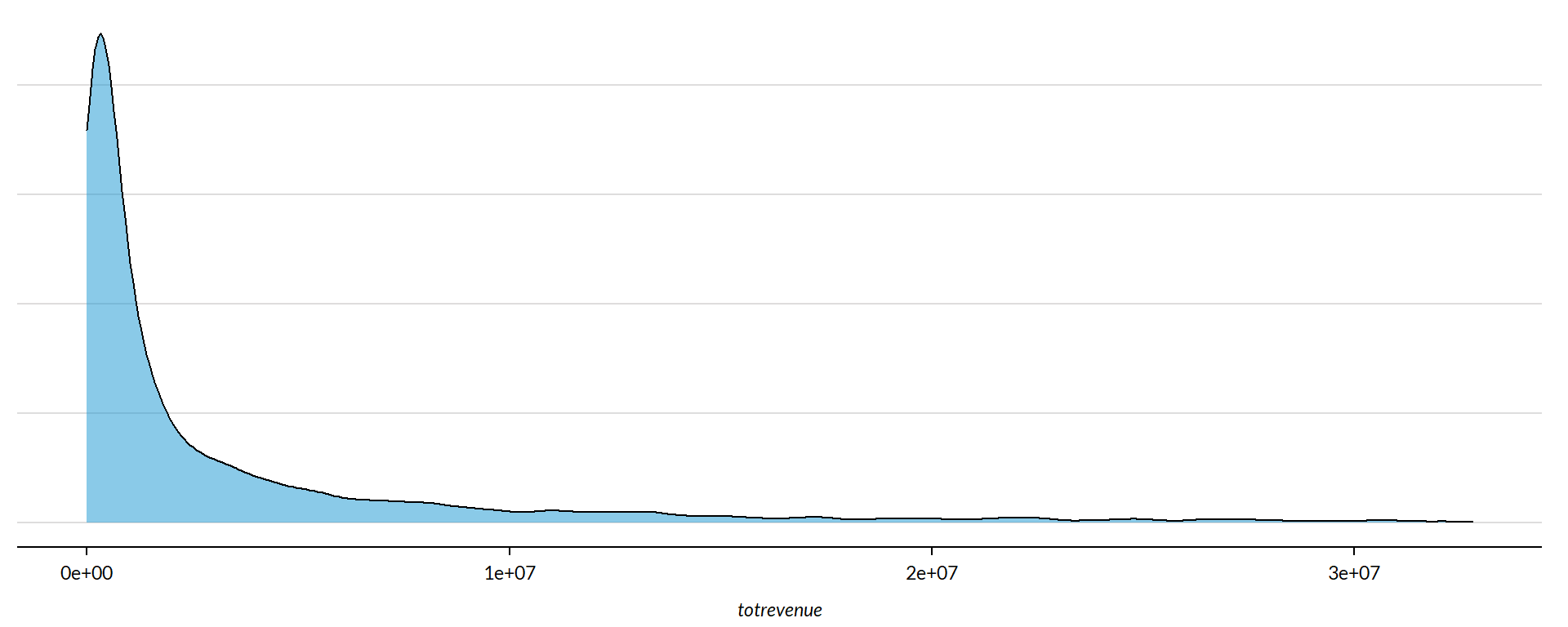
core2$totrevenue[ core2$totrevenue < 1 ] <- 1

if( nrow(core2) > 10000 )
{
  core3 <- sample_n( core2, 10000 )
} else
{
  core3 <- core2
}

jplot( log10(core3$totrevenue), core3$quick_ratio,
       xlab="Nonprofit Size (logged Revenue)",
       ylab=variable.label,
       xaxt="n", xlim=c(3,10) )
axis( side=1,
      at=c(3,4,5,6,7,8,9,10),
      labels=c("1k","10k","100k","1m","10m","100m","1b","10b") )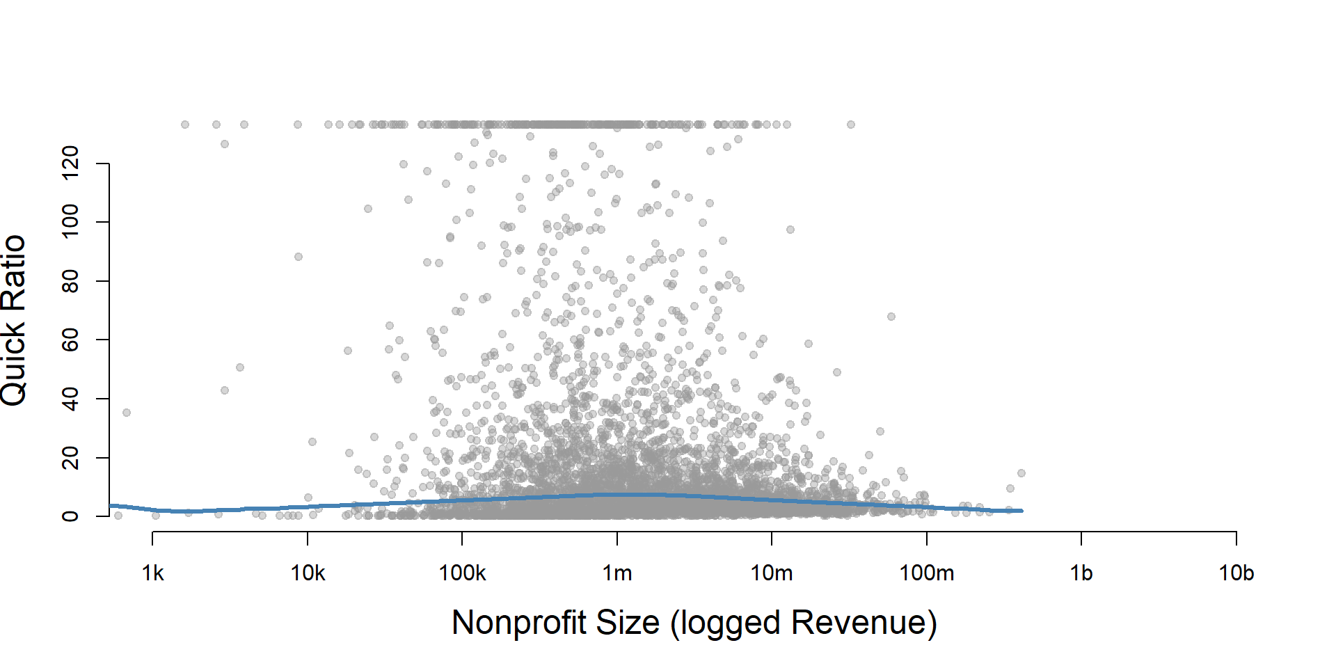
core2 %>%
  filter( ! is.na(rev.q) ) %>%
  ggplot( aes(quick_ratio) )  +
    geom_density( alpha = 0.5 ) +
    labs( title="Nonprofit Size (logged revenues)" ) +
    xlab( variable.label ) +
    facet_wrap( ~ rev.q, nrow=3 ) +
    theme_minimal( base_size = 22 )  +
    theme( axis.title.y=element_blank(),
           axis.text.y=element_blank(),
           axis.ticks.y=element_blank() )
Quick Ratio by Nonprofit Size (Net Assets)
ggplot( core2, aes(x = totnetassetend )) +
  geom_density( alpha = 0.5) +
  xlim( quantile(core2$totnetassetend, c(0.02,0.98), na.rm=T ) ) +
  xlab( "Net Assets" ) +
    theme( axis.title.y=element_blank(),
           axis.text.y=element_blank(),
           axis.ticks.y=element_blank() )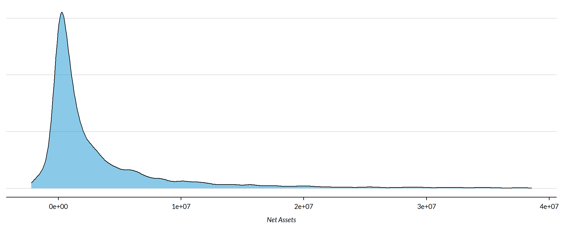
core2$totnetassetend[ core2$totnetassetend < 1 ] <- NA

if( nrow(core2) > 10000 )
{
  core3 <- sample_n( core2, 10000 )
} else
{
  core3 <- core2
}

jplot( log10(core3$totnetassetend), core3$quick_ratio,
       xlab="Nonprofit Size (logged Net Assets)",
       ylab=variable.label,
       xaxt="n", xlim=c(3,10) )
axis( side=1,
      at=c(3,4,5,6,7,8,9,10),
      labels=c("1k","10k","100k","1m","10m","100m","1b","10b") )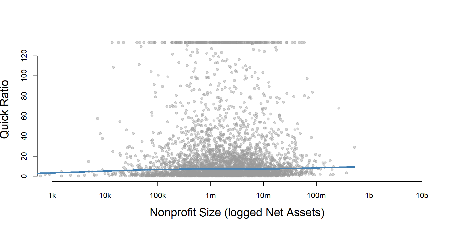
core2$totnetassetend[ core2$totnetassetend < 1 ] <- NA
core2$asset.q <- create_quantiles( var=core2$totnetassetend, n.groups=5 )

core2 %>%
  filter( ! is.na(asset.q) ) %>%
  ggplot( aes(quick_ratio) )  +
    geom_density( alpha = 0.5 ) +
    labs( title="Nonprofit Size (logged net assets, if assets > 0)" ) +
    xlab( variable.label ) +
    ylab( "" ) +
    facet_wrap( ~ asset.q, nrow=3 ) +
    theme_minimal( base_size = 22 )  +
    theme( axis.title.y=element_blank(),
           axis.text.y=element_blank(),
           axis.ticks.y=element_blank() )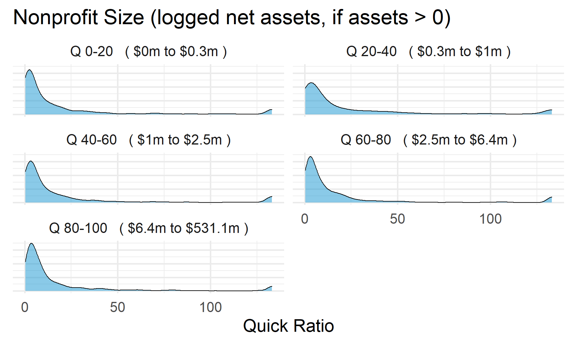
Total Assets for Comparison
core2$totassetsend[ core2$totassetsend < 1 ] <- NA
core2$tot.asset.q <- create_quantiles( var=core2$totassetsend, n.groups=5 )

if( nrow(core2) > 10000 )
{
  core3 <- sample_n( core2, 10000 )
} else
{
  core3 <- core2
}

jplot( log10(core3$totassetsend), core3$quick_ratio,
       xlab="Nonprofit Size (logged Total Assets)",
       ylab=variable.label,
       xaxt="n", xlim=c(3,10) )
axis( side=1,
      at=c(3,4,5,6,7,8,9,10),
      labels=c("1k","10k","100k","1m","10m","100m","1b","10b") )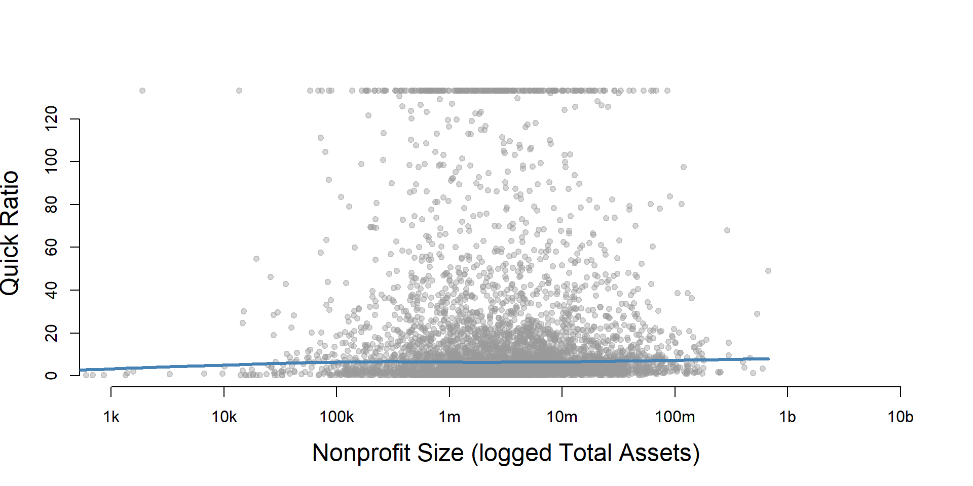
ggplot( core2, aes(x = totassetsend )) +
  geom_density( alpha = 0.5) +
  xlim( quantile(core2$totassetsend, c(0.02,0.98), na.rm=T ) ) +
  xlab( "Net Assets" ) +
    theme( axis.title.y=element_blank(),
           axis.text.y=element_blank(),
           axis.ticks.y=element_blank() )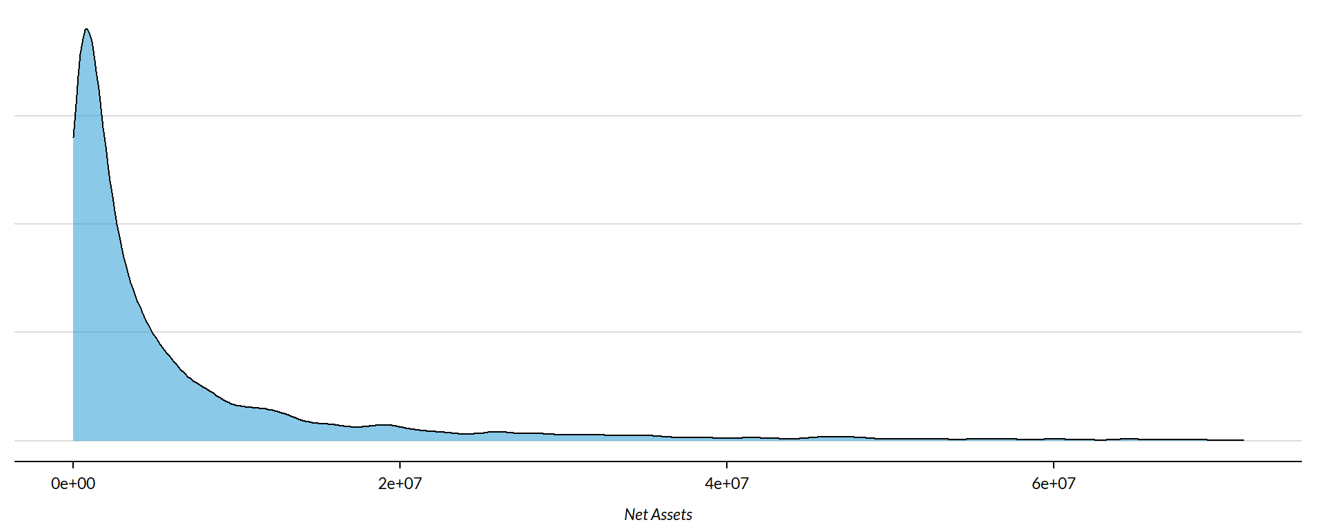
core2 %>%
  filter( ! is.na(tot.asset.q) ) %>%
  ggplot( aes(quick_ratio) )  +
    geom_density( alpha = 0.5 ) +
    xlab( "Nonprofit Size (logged total assets, if assets > 0)" ) +
    ylab( variable.label ) +
    facet_wrap( ~ tot.asset.q, nrow=3 ) +
    theme_minimal( base_size = 22 )  +
    theme( axis.title.y=element_blank(),
           axis.text.y=element_blank(),
           axis.ticks.y=element_blank() )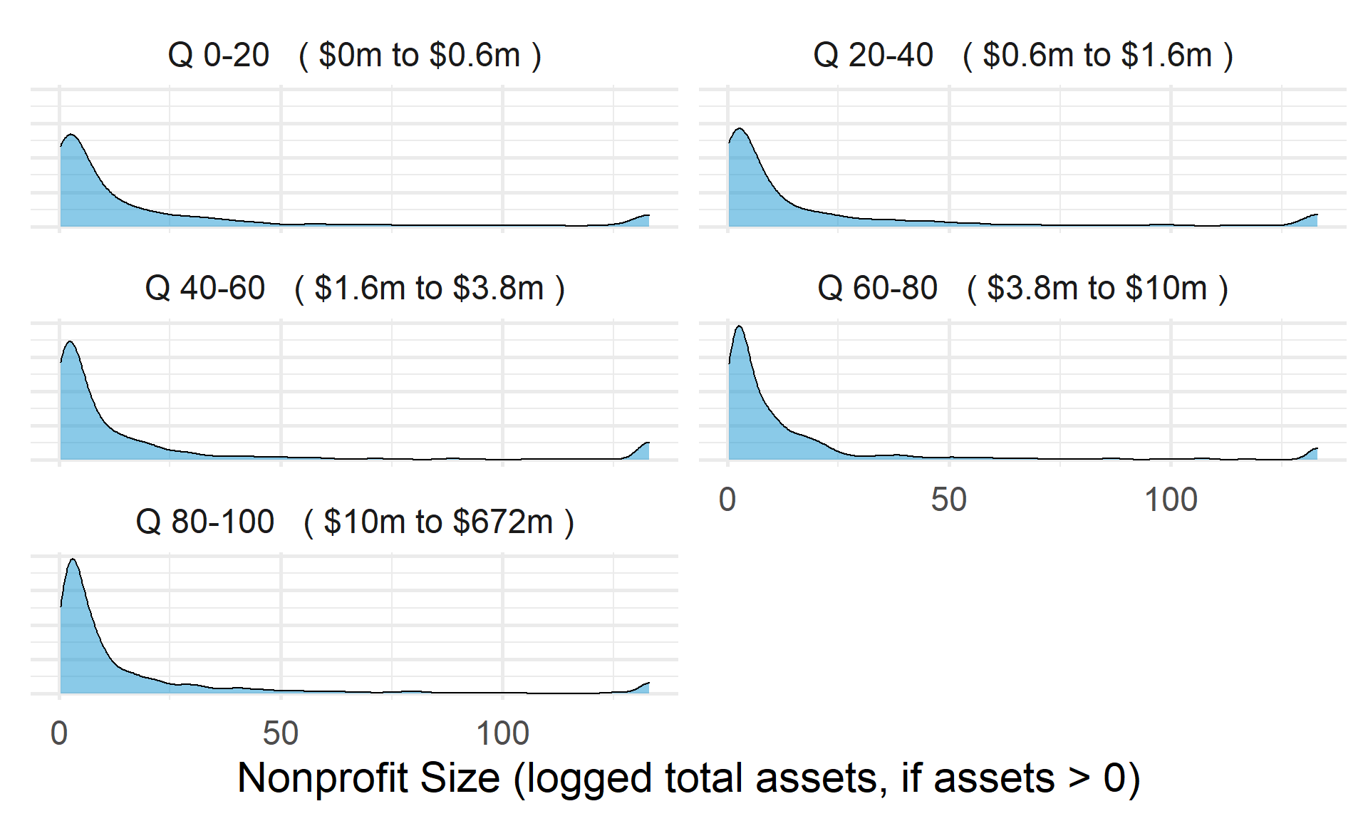
Quick Ratio by Nonprofit Age
ggplot( core2, aes(x = AGE )) +
geom_density( alpha = 0.5 ) 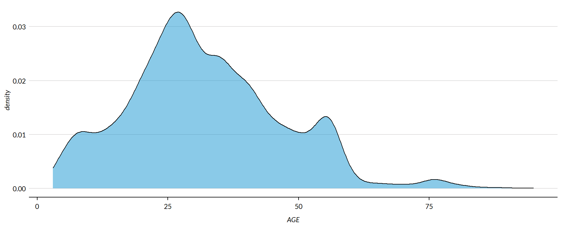
core2$AGE[ core2$AGE < 1 ] <- NA

if( nrow(core2) > 10000 )
{
  core3 <- sample_n( core2, 10000 )
} else
{
  core3 <- core2
}

jplot( core3$AGE, core3$quick_ratio,
       xlab="Nonprofit Age",
ylab=variable.label ) 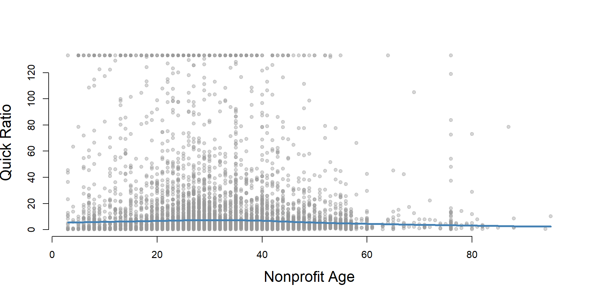
core2 %>%
  filter( ! is.na(age.q) ) %>%
  ggplot( aes(quick_ratio) )  +
    geom_density( alpha = 0.5 ) +
    labs( title="Nonprofit Age" ) +
    xlab( variable.label ) +
    ylab( "" ) +
    facet_wrap( ~ age.q, nrow=3 ) +
    theme_minimal( base_size = 22 )  +
    theme( axis.title.y=element_blank(),
           axis.text.y=element_blank(),
           axis.ticks.y=element_blank() )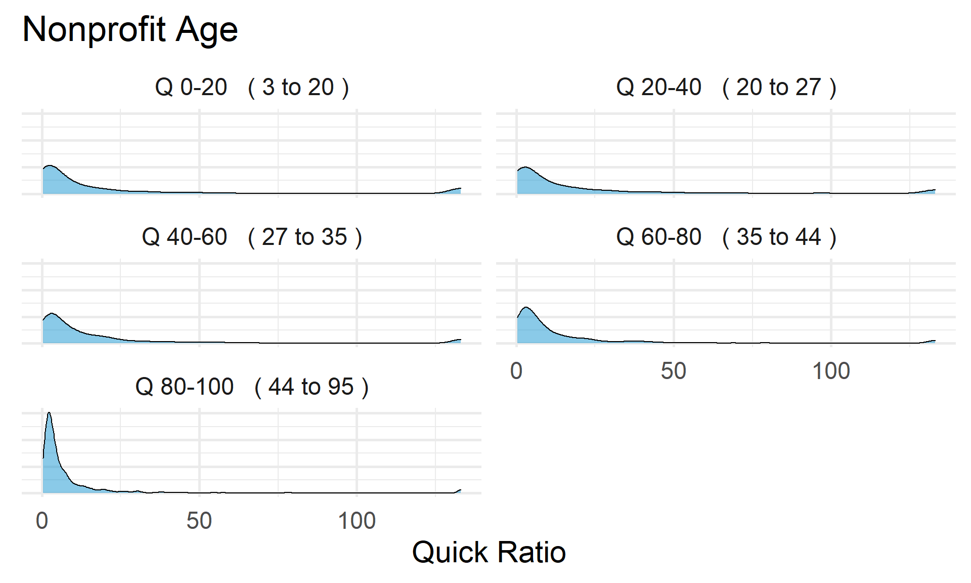
Quick Ratio by Land and Building Value
ggplot( core2, aes(x = lndbldgsequipend )) +
geom_density( alpha = 0.5 ) 
core2$lndbldgsequipend[ core2$lndbldgsequipend < 1 ] <- NA

if( nrow(core2) > 10000 )
{
  core3 <- sample_n( core2, 10000 )
} else
{
  core3 <- core2


jplot( log10(core3$lndbldgsequipend), core3$quick_ratio,
       xlab="Land and Building Value (logged)",
       ylab=variable.label,
       xaxt="n", xlim=c(3,10) )
axis( side=1,
      at=c(3,4,5,6,7,8,9,10),
      labels=c("1k","10k","100k","1m","10m","100m","1b","10b") )
}
core2 %>%
  filter( ! is.na(land.q) ) %>%
  ggplot( aes(quick_ratio) )  +
    geom_density( alpha = 0.5 ) +
    labs( title="Land and Building Value" ) +
    xlab( variable.label ) +
    ylab( "" ) +
    facet_wrap( ~ land.q, nrow=3 ) +
    theme_minimal( base_size = 22 )  +
    theme( axis.title.y=element_blank(),
           axis.text.y=element_blank(),
           axis.ticks.y=element_blank() )
Save Metrics
core.quick_ratio <- select( core, ein, tax_pd, quick_ratio )
saveRDS( core.quick_ratio, "03-data-ratios/m-12-quick-ratio.rds" )
write.csv( core.quick_ratio, "03-data-ratios/m-12-quick-ratio.csv" )