Metric Construction

Definition & Interpretation

There are three indicators to construct that show the relationship between types of income to overall revenue, and one final indicator that analyzes across all three of those indicators, picking the largest of them for any organization, which ultimately shows what the average degree of dependence on any one source of income is across all organizations.

Donation/Grant Dependence Ratio

\[Donation/Grant\: Dependence \:Ratio = \frac{Donation\: or \: Grant\: Revenues}{Total \: Revenues} \]

This metric shows how much of an organization’s total revenues come from contributions, government grants, and special event reveues. High levels in this indicator are undesirable since that means that an organization’s revenues are volatile insofar as it is dependent on contributions that are highly likely to contract during economic downturns. Low values in this indicator mean an organization is not dependent on donations.

### Earned Income Dependence Ratio \[Earned\: Income\: Dependence \:Ratio = \frac{Earned\: Income}{Total \: Revenues} \]

This metric shows how much of an organization’s total revenues come from earned income (program service revenues, dues, assessments, profits from sales). High levels in this indicator are more desirable since that means that an organization is fairly self-sustaining with its own activities. Low values in this indicator mean an organization is likely dependent on donations or investments for their revenues and thus more vulnerable to the sentiments of donors or market forces.

Investment Income Dependence Ratio

\[Investment\: Income\: Dependence \:Ratio = \frac{Investment\: Income}{Total \: Revenues} \]

This metric shows how much of an organization’s total revenues come from investment income (interest, dividents, gains/losses on sales of securities or other assets). High levels in this metric indicate an organization is more depenent on investment income (and thus vulnerable to market downturns), and low values indicate their income comes more from donations or earned income.

Income Reliance Ratio

\[Income \:Reliance \:Ratio = Max({Investment\: Income \:Ratio,\: Donation \: Dependence \: Ratio,\: Earned \: Income \: Ratio) \]

This metric shows on average how much organizations depend on a single source of revenue.

This metric is limited because it doesn’t indicate which source of revenue organizations are dependent on. Given that high values in the donation and investment ratios indicate vulnerability to market downturns while high values in the earned income ratio indicate financial independence, interpretation of this variable must be restricted to simply understanding business models.

Variables

Note: This data is available only for organizations that file full 990s. [Organizations with revenues <$200,000 and total assets <$500,000 have the option to not file a full 990 and file an EZ instead.]

Donation/Grant Dependence Ratio

Numerator: Donation Revenues [total contributions and net special event revenue]
- On 990: Part VIII, Line 1h(A) + Part VIII, Line 8c(A)
  - SOI PC EXTRACTS: (totcntrbgfts+netincfndrsng)
- On EZ: Not Available
  - SOI PC EXTRACTS: Not Available
Denominator: Total Reveues
- On 990: (Part VIII, Line 12A) -SOI PC EXTRACTS: totrevenue
- On EZ: Part I, Line 9 -SOI PC EXTRACTS: totrevnue

Earned Income Dependence Ratio

Numerator: Earned income (program service revenue, royalties, profits from sale of inventory, and other revenue)
- On 990: (Part VIII, Line 2g(A)) + (Part VIII, Line 1b(A)) + (Part VIII, Line 5(A)) + (Part VIII, Line 11d(A))
  - SOI PC EXTRACTS: (totprgmrevnue +royaltsinc+ netincsales+miscrevtot11e)
- On EZ: Not Available
  - SOI PC EXTRACTS: Not Available
Denominator: Total Reveues
- On 990: (Part VIII, Line 12A) -SOI PC EXTRACTS: totrevenue
- On EZ: Part I, Line 9 -SOI PC EXTRACTS: totrevnue

Investment Income Dependence Ratio

Numerator: Investment income (interest, dividends, net rental income, and realized gains/losses on sales of securities or other assets)
- On 990: (Part VIII, Line 3(A)) + (Part VIII, Line 4(A)) + (Part VIII, Line 6(A)) + (Part VIII, Line 7(A))
  - SOI PC EXTRACTS: (invstmntinc + txexmptbndsproceeds + netrntlinc + netgnls)
- On EZ: Not Available
  - SOI PC EXTRACTS: Not Available
Denominator: Total Reveues
- On 990: (Part VIII, Line 12A) -SOI PC EXTRACTS: totrevenue
- On EZ: Part I, Line 9 -SOI PC EXTRACTS: totrevnue

Donation/Grant Reliance Ratio Analysis

# TEMPORARY VARIABLES 
donation_revenues  <- core$totcntrbgfts + core$netincfndrsng
totalrevenues <- ( core$totrevenue )

# can't divide by zero
totalrevenues[ totalrevenues == 0 ] <- NA

# SAVE RESULTS 
core$donation_ratio <-  donation_revenues / totalrevenues
                     
# summary( core$donation_ratio )

Standardize Scales

Check high and low values to see what makes sense.

x.05 <- quantile( core$donation_ratio, 0.05, na.rm=T )
x.95 <- quantile( core$donation_ratio, 0.95, na.rm=T )

ggplot( core, aes(x = donation_ratio ) ) +  
  geom_density( alpha = 0.5) + 
  xlim( x.05, x.95 )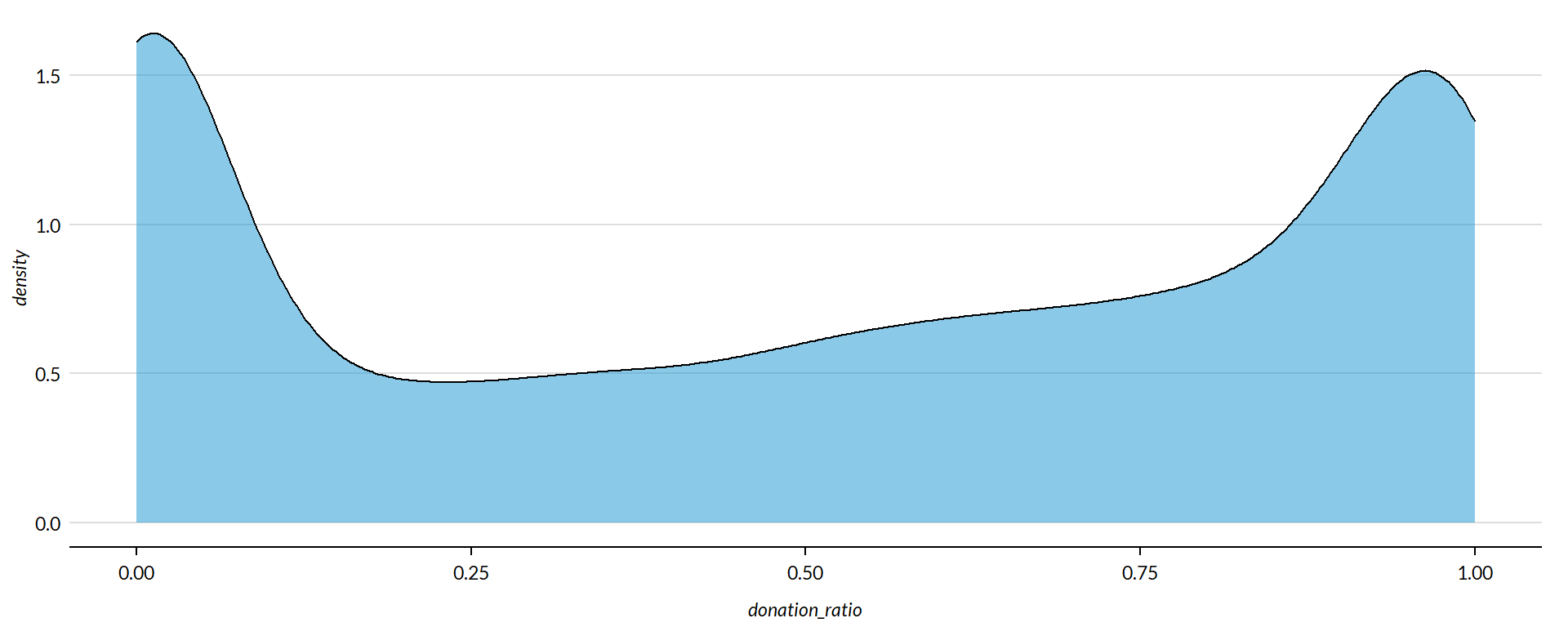

core2 <- core

# proportion of values that are negative
#mean( core2$donation_ratio < 0, na.rm=T ) 
#core2$donation_ratio[ core2$donation_ratio < 0 ] <- 0

# proption of values above 200% 
#mean( core2$donation_ratio > 50, na.rm=T ) 
#core2$donation_ratio[ core2$donation_ratio > 50 ] <- 50



x.05 <- quantile( core$donation_ratio, 0.05, na.rm=T )
x.95 <- quantile( core$donation_ratio, 0.95, na.rm=T )

core2 <- core

# proportion of values that are negative
# mean( core2$der < 0, na.rm=T ) 

# proption of values above 1% 
# mean( core2$der > 5, na.rm=T ) 

# WINSORIZATION AT 5th and 95th PERCENTILES

core2$donation_ratio[ core2$donation_ratio < x.05 ] <- x.05
core2$donation_ratio[ core2$donation_ratio > x.95 ] <- x.95

Metric Scope

Tax data is available for full 990 filers only, so this metric does not describe any organizations with Gross receipts < $200,000 and Total assets < $500,000. Some organizations with receipts or assets below those thresholds may have filed a full 990, but these would be exceptions.

The data have been capped to those with values between 5% and 95% of the normal distribution to cut off outliers and exempt organizations with zero profitability (though negative values are allowed still).

Descriptive Statistics

Note: All monetary variables have been converted to thousands of dollars. Metric has been scaled/multiplied by 100 for readability.


core2 %>%
  mutate( donation_ratio = donation_ratio * 100,
    totrevenue = totrevenue / 1000,
    totfuncexpns = totfuncexpns / 1000, 
    lndbldgsequipend = lndbldgsequipend / 1000,
    totassetsend = totassetsend / 1000,
    totliabend = totliabend / 1000,
    totnetassetend = totnetassetend / 1000 ) %>% 
  select( STATE,  NTEE1, NTMAJ12, 
          donation_ratio, 
          AGE, 
          totrevenue, totfuncexpns, 
          lndbldgsequipend, totassetsend, 
          totnetassetend, totliabend ) %>%

  stargazer( type = s.type, 
             digits=2, 
             summary.stat = c("min","p25","median",
                              "mean","p75","max", "sd"),
             covariate.labels = c("Donation/Grant Reliance Ratio", "Age", 
                                  "Revenue ($1k)", "Expenses($1k)", 
                                  "Buildings ($1k)", "Total Assets ($1k)",
                                  "Net Assets ($1k)", "Liabiliies ($1k)"))


Statistic	Min	Pctl(25)	Median	Mean	Pctl(75)	Max	St. Dev.

Donation/Grant Reliance Ratio	0.00	7.33	56.36	51.41	90.41	100.00	38.21
Age	3	22	30	32.04	41	95	14.75
Revenue (1k)	-5,376.77	258.90	909.40	4,521.71	3,672.25	408,932.00	14,285.64
Expenses(1k)	0.00	263.50	840.06	4,192.08	3,327.50	382,666.50	13,465.77
Buildings (1k)	-4.48	79.14	824.25	3,504.47	2,868.50	513,508.80	13,210.06
Total Assets (1k)	-7,552.11	777.90	2,446.11	9,261.85	7,477.25	672,021.00	27,038.89
Net Assets (1k)	-178,869.70	155.67	1,093.86	4,553.27	4,078.70	531,067.70	15,470.31
Liabiliies (1k)	-2,707.10	115.44	815.58	4,708.51	3,133.16	705,623.10	18,721.86

What proportion of orgs have Donation/Grant Reliance Ratios equal to zero?

prop.zero <- mean( core2$donation_ratio == 0, na.rm=T )

In the sample, 17 percent of the organizations have Donation/Grant Reliance Ratios equal to zero, meaning they have no donation revenues. These organizations are dropped from subsequent graphs to keep the visualizations clean. The interpretation of the graphics should be the distributions of Donation/Grant Reliance Ratios for organizations that have positive or negative values.

###
### ADD QUANTILES
###
###   function create_quantiles() defined in r-functions.R

core2$exp.q   <- create_quantiles( var=core2$totfuncexpns,   n.groups=5 )
core2$rev.q   <- create_quantiles( var=core2$totrevenue,     n.groups=5 )
core2$asset.q <- create_quantiles( var=core2$totnetassetend, n.groups=5 )
core2$age.q   <- create_quantiles( var=core2$AGE,            n.groups=5 )
core2$land.q   <- create_quantiles( var=core2$lndbldgsequipend,  n.groups=5 )

Donated Income Dependence Ratio Density

min.x <- min( core2$donation_ratio, na.rm=T )
max.x <- max( core2$donation_ratio, na.rm=T )

ggplot( core2, aes(x = donation_ratio )) +  
  geom_density( alpha = 0.5 ) + 
  xlim( min.x, max.x  ) +
  xlab( variable.label1 ) +
  theme( axis.title.y=element_blank(),
         axis.text.y=element_blank(), 
         axis.ticks.y=element_blank() )

Donated Income Dependence Ratio by NTEE Major Code

core3 <- core2 %>% filter( ! is.na(NTEE1) )
table( core3$NTEE1) %>% sort(decreasing=TRUE) %>% kable()

Var1	Freq
Housing	2837
Community Development	1585
Human Services	1102


t <- table( factor(core3$NTEE1) ) 
df <- data.frame( x=Inf, y=Inf, 
                  N=paste0( "N=", as.character(t) ), 
                  NTEE1=names(t) )

ggplot( core3, aes( x=donation_ratio ) ) + 
  geom_density( alpha = 0.5) + 
  # xlim( -0.1, 1 ) +
  labs( title="Nonprofit Subsectors" ) + 
  xlab( variable.label1 ) + 
  facet_wrap( ~ NTEE1, nrow=1 ) + 
    theme_minimal( base_size = 15 )  + 
    theme( axis.title.y=element_blank(),
           axis.text.y=element_blank(), 
           axis.ticks.y=element_blank(),
           strip.text = element_text( face="bold") ) +  # size=20 
  geom_text( data=df, 
             aes(x, y, label=N ), 
             hjust=2, vjust=3, 
             color="gray60", size=6 )

Donated Income Dependence Ratio by Region

table( core2$Region) %>% kable()

Var1	Freq
Midwest	1444
Northeast	1368
South	1610
West	1088

t <- table( factor(core2$Region) ) 
df <- data.frame( x=Inf, y=Inf, 
                  N=paste0( "N=", as.character(t) ), 
                  Region=names(t) )

core2 %>% 
  filter( ! is.na(Region) ) %>% 
  ggplot( aes(donation_ratio) )  + 
    geom_density( alpha = 0.5 ) + 
    xlab( "Census Regions" ) + 
    ylab( variable.label1 ) +
    facet_wrap( ~ Region, nrow=3 ) + 
    theme_minimal( base_size = 22 )  + 
    theme( axis.title.y=element_blank(),
           axis.text.y=element_blank(), 
           axis.ticks.y=element_blank() ) + 
    geom_text( data=df, 
             aes(x, y, label=N ), 
             hjust=2, vjust=3, 
             color="gray60", size=6 )

table( core2$Division ) %>% kable()

Var1	Freq
East North Central	1038
East South Central	289
Middle Atlantic	904
Mountain	303
New England	464
Pacific	785
South Atlantic	900
West North Central	406
West South Central	421

t <- table( factor(core2$Division) ) 
df <- data.frame( x=Inf, y=Inf, 
                  N=paste0( "N=", as.character(t) ), 
                  Division=names(t) )

core2 %>% 
  filter( ! is.na(Division) ) %>% 
  ggplot( aes(donation_ratio) )  + 
    geom_density( alpha = 0.5 ) + 
    xlab( "Census Sub-Regions (10)" ) + 
    ylab( variable.label1 ) +
    facet_wrap( ~ Division, nrow=3 ) + 
    theme_minimal( base_size = 22 )  + 
    theme( axis.title.y=element_blank(),
           axis.text.y=element_blank(), 
           axis.ticks.y=element_blank() ) + 
    geom_text( data=df, 
             aes(x, y, label=N ), 
             hjust=2, vjust=3, 
             color="gray60", size=6 )

Donated Income Dependence Ratio by Nonprofit Size (Expenses)

ggplot( core2, aes(x = totfuncexpns )) +  
  geom_density( alpha = 0.5 ) + 
  xlim( quantile(core2$totfuncexpns, c(0.02,0.98), na.rm=T ) )

core2$totfuncexpns[ core2$totfuncexpns < 1 ] <- 1
# core2$totfuncexpns[ is.na(core2$totfuncexpns) ] <- 1

if( nrow(core2) > 10000 )
{
  core3 <- sample_n( core2, 10000 )
} else
{
  core3 <- core2
}

jplot( log10(core3$totfuncexpns), core3$donation_ratio, 
       xlab="Nonprofit Size (logged Expenses)", 
       ylab=variable.label1,
       xaxt="n", xlim=c(3,10) )
axis( side=1, 
      at=c(3,4,5,6,7,8,9,10), 
      labels=c("1k","10k","100k","1m","10m","100m","1b","10b") )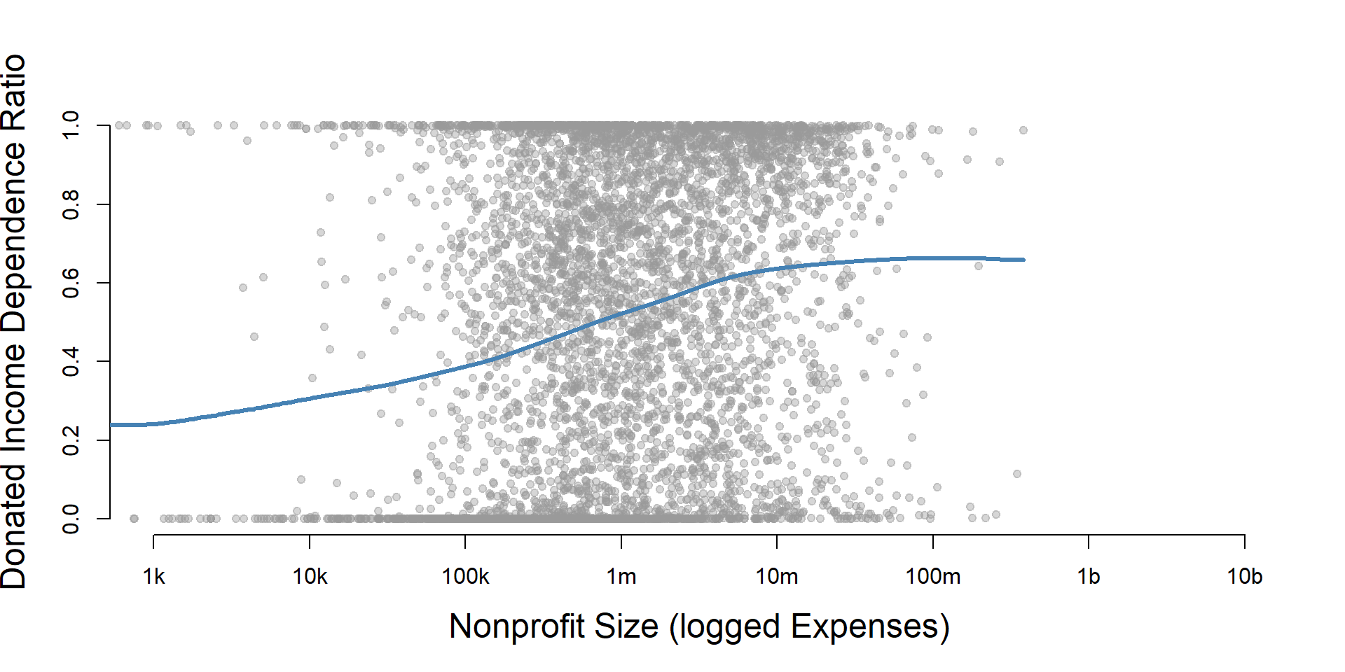

core2 %>% 
  filter( ! is.na(exp.q) ) %>% 
  ggplot( aes(donation_ratio) )  + 
    geom_density( alpha = 0.5) + 
    labs( title="Nonprofit Size (logged expenses)" ) + 
    xlab( variable.label1 ) +
    facet_wrap( ~ exp.q, nrow=3 ) + 
    theme_minimal( base_size = 22 )  + 
    theme( axis.title.y=element_blank(),
           axis.text.y=element_blank(), 
           axis.ticks.y=element_blank() )

Donated Income Dependence Ratio by Nonprofit Size (Revenue)

ggplot( core2, aes(x = totrevenue )) +  
  geom_density( alpha = 0.5 ) + 
  xlim( quantile(core2$totrevenue, c(0.02,0.98), na.rm=T ) ) + 
  theme( axis.title.y=element_blank(),
           axis.text.y=element_blank(), 
           axis.ticks.y=element_blank() )

core2$totrevenue[ core2$totrevenue < 1 ] <- 1

if( nrow(core2) > 10000 )
{
  core3 <- sample_n( core2, 10000 )
} else
{
  core3 <- core2
}

jplot( log10(core3$totrevenue), core3$donation_ratio, 
       xlab="Nonprofit Size (logged Revenue)", 
       ylab=variable.label1,
       xaxt="n", xlim=c(3,10) )
axis( side=1, 
      at=c(3,4,5,6,7,8,9,10), 
      labels=c("1k","10k","100k","1m","10m","100m","1b","10b") )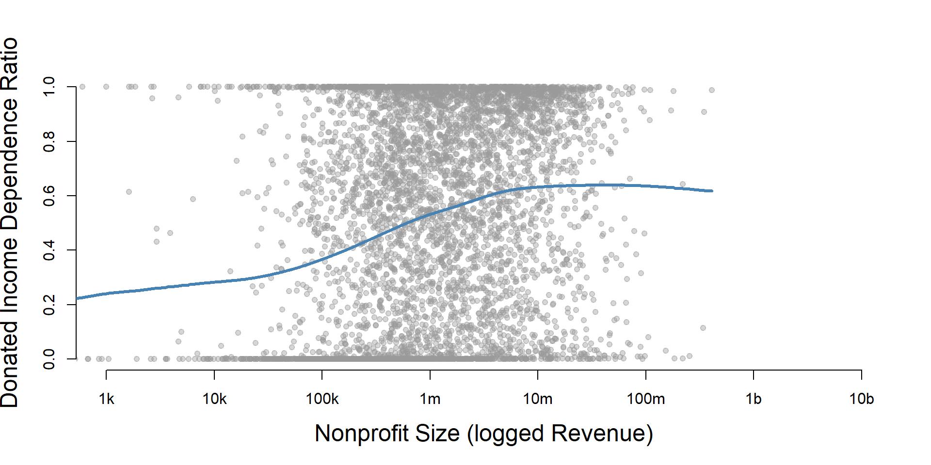

core2 %>% 
  filter( ! is.na(rev.q) ) %>% 
  ggplot( aes(donation_ratio) )  + 
    geom_density( alpha = 0.5 ) + 
    labs( title="Nonprofit Size (logged revenues)" ) + 
    xlab( variable.label1 ) +
    facet_wrap( ~ rev.q, nrow=3 ) + 
    theme_minimal( base_size = 22 )  + 
    theme( axis.title.y=element_blank(),
           axis.text.y=element_blank(), 
           axis.ticks.y=element_blank() )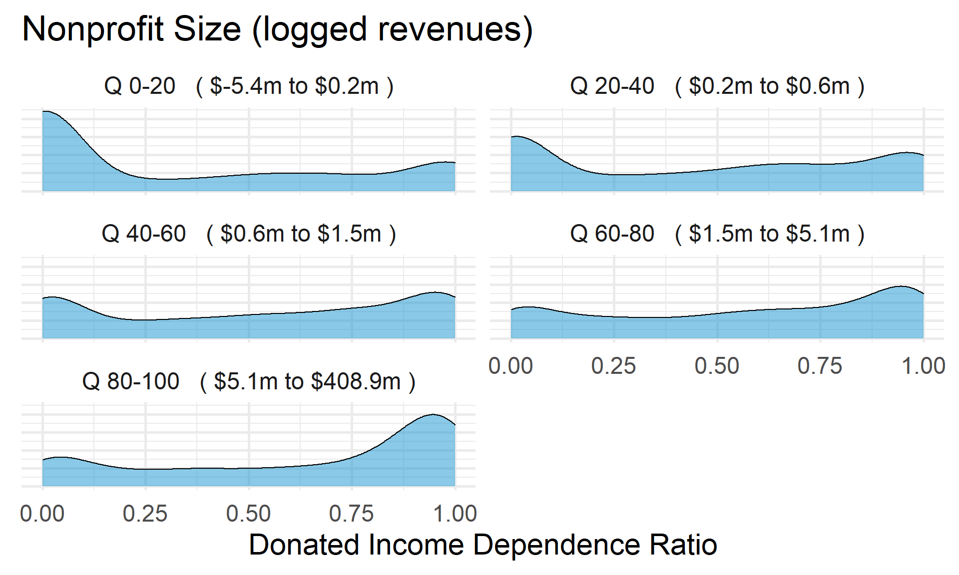

Donated Income Dependence Ratio by Nonprofit Size (Net Assets)

ggplot( core2, aes(x = totnetassetend )) +  
  geom_density( alpha = 0.5) + 
  xlim( quantile(core2$totnetassetend, c(0.02,0.98), na.rm=T ) ) + 
  xlab( "Net Assets" ) +
    theme( axis.title.y=element_blank(),
           axis.text.y=element_blank(), 
           axis.ticks.y=element_blank() )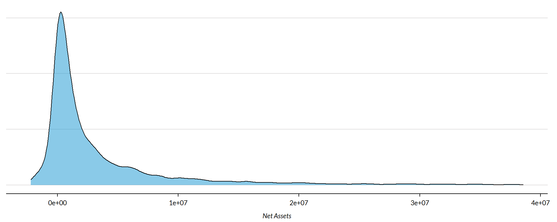

core2$totnetassetend[ core2$totnetassetend < 1 ] <- NA

if( nrow(core2) > 10000 )
{
  core3 <- sample_n( core2, 10000 )
} else
{
  core3 <- core2
}

jplot( log10(core3$totnetassetend), core3$donation_ratio, 
       xlab="Nonprofit Size (logged Net Assets)", 
       ylab=variable.label1,
       xaxt="n", xlim=c(3,10) )
axis( side=1, 
      at=c(3,4,5,6,7,8,9,10), 
      labels=c("1k","10k","100k","1m","10m","100m","1b","10b") )

core2$totnetassetend[ core2$totnetassetend < 1 ] <- NA
core2$asset.q <- create_quantiles( var=core2$totnetassetend, n.groups=5 )

core2 %>% 
  filter( ! is.na(asset.q) ) %>% 
  ggplot( aes(donation_ratio) )  + 
    geom_density( alpha = 0.5 ) + 
    labs( title="Nonprofit Size (logged net assets, if assets > 0)" ) + 
    xlab( variable.label1 ) + 
    ylab( "" ) + 
    facet_wrap( ~ asset.q, nrow=3 ) + 
    theme_minimal( base_size = 22 )  + 
    theme( axis.title.y=element_blank(),
           axis.text.y=element_blank(), 
           axis.ticks.y=element_blank() )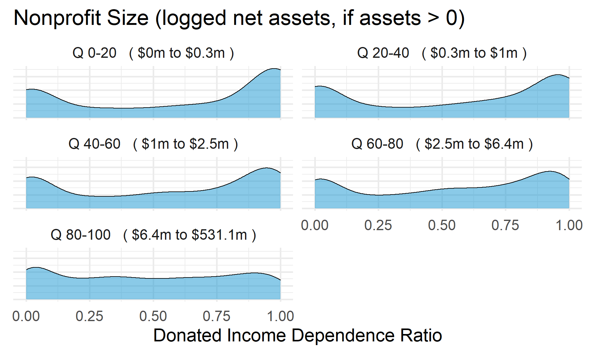

Total Assets for Comparison

core2$totassetsend[ core2$totassetsend < 1 ] <- NA
core2$tot.asset.q <- create_quantiles( var=core2$totassetsend, n.groups=5 )

if( nrow(core2) > 10000 )
{
  core3 <- sample_n( core2, 10000 )
} else
{
  core3 <- core2
}

jplot( log10(core3$totassetsend), core3$donation_ratio, 
       xlab="Nonprofit Size (logged Total Assets)", 
       ylab=variable.label1,
       xaxt="n", xlim=c(3,10) )
axis( side=1, 
      at=c(3,4,5,6,7,8,9,10), 
      labels=c("1k","10k","100k","1m","10m","100m","1b","10b") )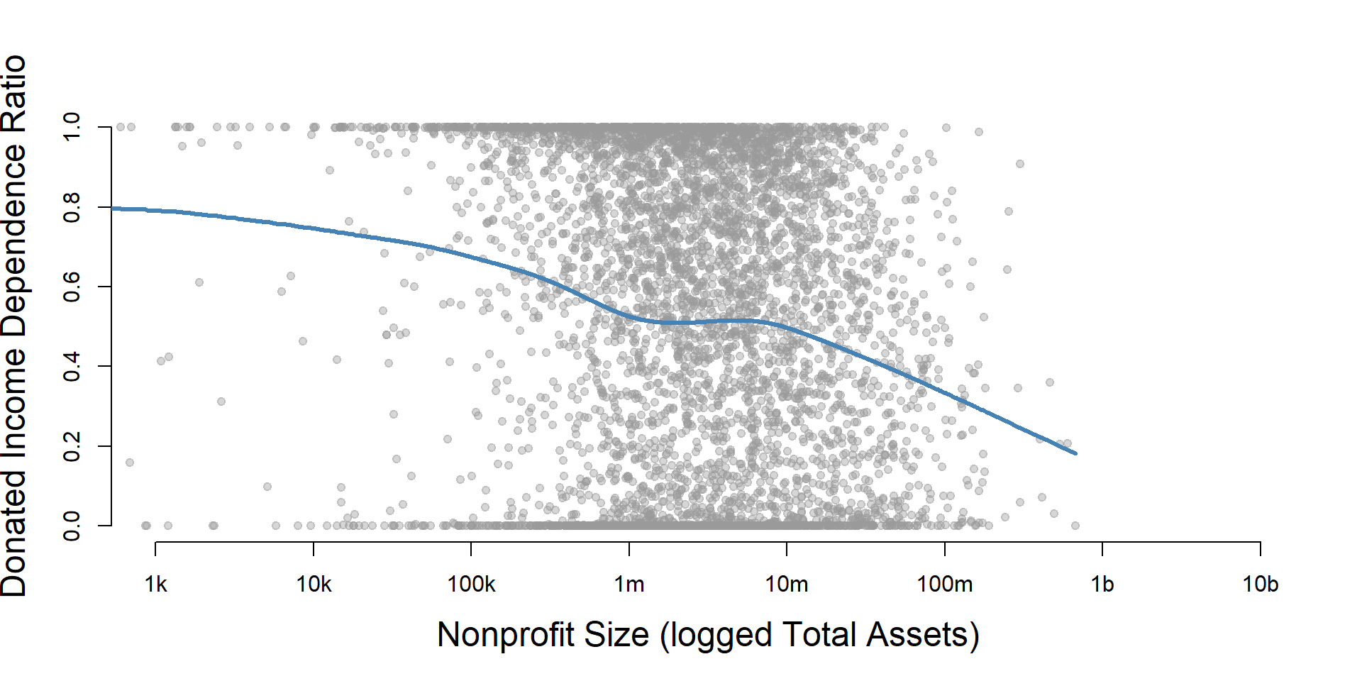

ggplot( core2, aes(x = totassetsend )) +  
  geom_density( alpha = 0.5) + 
  xlim( quantile(core2$totassetsend, c(0.02,0.98), na.rm=T ) ) + 
  xlab( "Net Assets" ) +
    theme( axis.title.y=element_blank(),
           axis.text.y=element_blank(), 
           axis.ticks.y=element_blank() )

core2 %>% 
  filter( ! is.na(tot.asset.q) ) %>% 
  ggplot( aes(donation_ratio) )  + 
    geom_density( alpha = 0.5 ) + 
    xlab( "Nonprofit Size (logged total assets, if assets > 0)" ) + 
    ylab( variable.label1 ) +
    facet_wrap( ~ tot.asset.q, nrow=3 ) + 
    theme_minimal( base_size = 22 )  + 
    theme( axis.title.y=element_blank(),
           axis.text.y=element_blank(), 
           axis.ticks.y=element_blank() )

Donated Income Dependence Ratio by Nonprofit Age

ggplot( core2, aes(x = AGE )) +  
  geom_density( alpha = 0.5 )

core2$AGE[ core2$AGE < 1 ] <- NA

if( nrow(core2) > 10000 )
{
  core3 <- sample_n( core2, 10000 )
} else
{
  core3 <- core2
}

jplot( core3$AGE, core3$donation_ratio, 
       xlab="Nonprofit Age", 
       ylab=variable.label1 )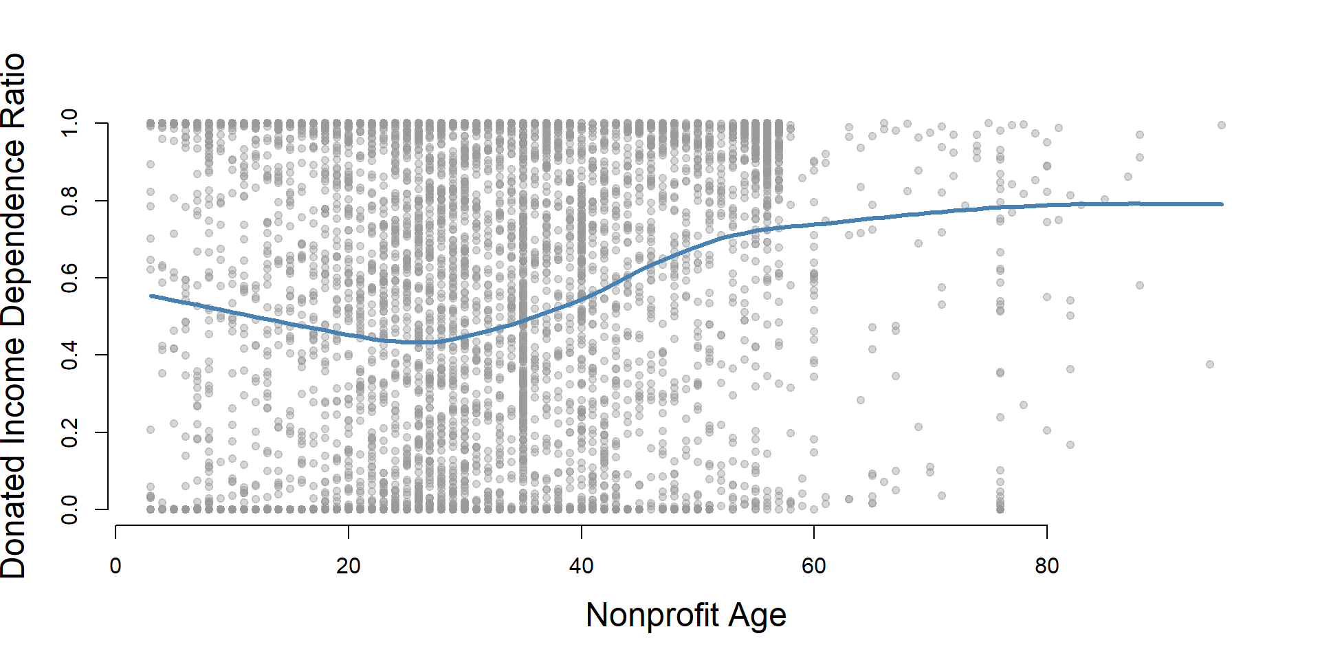

core2 %>% 
  filter( ! is.na(age.q) ) %>% 
  ggplot( aes(donation_ratio) )  + 
    geom_density( alpha = 0.5 ) + 
    labs( title="Nonprofit Age" ) + 
    xlab( variable.label1 ) +
    ylab( "" ) +
    facet_wrap( ~ age.q, nrow=3 ) + 
    theme_minimal( base_size = 22 )  + 
    theme( axis.title.y=element_blank(),
           axis.text.y=element_blank(), 
           axis.ticks.y=element_blank() )

Donated Income Dependence Ratio by Land and Building Value

ggplot( core2, aes(x = lndbldgsequipend )) +  
  geom_density( alpha = 0.5 )

core2$lndbldgsequipend[ core2$lndbldgsequipend < 1 ] <- NA
if( nrow(core2) > 10000 )
{
  core3 <- sample_n( core2, 10000 )
} else
{
  core3 <- core2


jplot( log10(core3$lndbldgsequipend), core3$donation_ratio, 
       xlab="Land and Building Value (logged)", 
       ylab=variable.label1,
       xaxt="n", xlim=c(3,10) )
axis( side=1, 
      at=c(3,4,5,6,7,8,9,10), 
      labels=c("1k","10k","100k","1m","10m","100m","1b","10b") )
}

core2 %>% 
  filter( ! is.na(land.q) ) %>% 
  ggplot( aes(donation_ratio) )  + 
    geom_density( alpha = 0.5 ) + 
    labs( title="Land and Building Value" ) + 
    xlab( variable.label1 ) +
    ylab( "" ) +
    facet_wrap( ~ land.q, nrow=3 ) + 
    theme_minimal( base_size = 22 )  + 
    theme( axis.title.y=element_blank(),
           axis.text.y=element_blank(), 
           axis.ticks.y=element_blank() )

Earned Income Reliance Ratio Analysis

# TEMPORARY VARIABLES 
earned_income  <- core$totprgmrevnue +core$royaltsinc+ core$netincsales+core$miscrevtot11e 
totalrevenues <- ( core$totrevenue )

# can't divide by zero
totalrevenues[ totalrevenues == 0 ] <- NA

# SAVE RESULTS 
core$earned_income_ratio <-  earned_income / totalrevenues
                     
# summary( core$earned_income_ratio )

Standardize Scales

Check high and low values to see what makes sense.

x.05 <- quantile( core$earned_income_ratio, 0.05, na.rm=T )
x.95 <- quantile( core$earned_income_ratio, 0.95, na.rm=T )

ggplot( core, aes(x = earned_income_ratio ) ) +  
  geom_density( alpha = 0.5) + 
  xlim( x.05, x.95 )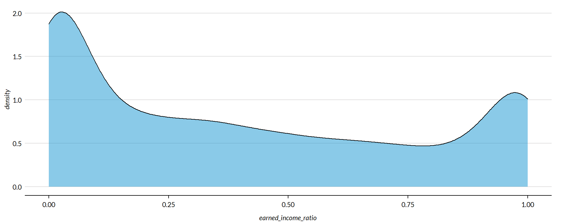

core2 <- core

# proportion of values that are negative
#mean( core2$earned_income_ratio < 0, na.rm=T ) 
#core2$earned_income_ratio[ core2$earned_income_ratio < 0 ] <- 0

# proption of values above 200% 
#mean( core2$earned_income_ratio > 50, na.rm=T ) 
#core2$earned_income_ratio[ core2$earned_income_ratio > 50 ] <- 50



x.05 <- quantile( core$earned_income_ratio, 0.05, na.rm=T )
x.95 <- quantile( core$earned_income_ratio, 0.95, na.rm=T )

core2 <- core

# proportion of values that are negative
# mean( core2$der < 0, na.rm=T ) 

# proption of values above 1% 
# mean( core2$der > 5, na.rm=T ) 

# WINSORIZATION AT 5th and 95th PERCENTILES

core2$earned_income_ratio[ core2$earned_income_ratio < x.05 ] <- x.05
core2$earned_income_ratio[ core2$earned_income_ratio > x.95 ] <- x.95

Metric Scope

Descriptive Statistics

Note: All monetary variables have been converted to thousands of dollars.


core2 %>%
  mutate( # earned_income_ratio = earned_income_ratio * 10000,
    totrevenue = totrevenue / 1000,
    totfuncexpns = totfuncexpns / 1000, 
    lndbldgsequipend = lndbldgsequipend / 1000,
    totassetsend = totassetsend / 1000,
    totliabend = totliabend / 1000,
    totnetassetend = totnetassetend / 1000 ) %>% 
  select( STATE,  NTEE1, NTMAJ12, 
          earned_income_ratio, 
          AGE, 
          totrevenue, totfuncexpns, 
          lndbldgsequipend, totassetsend, 
          totnetassetend, totliabend ) %>%

  stargazer( type = s.type, 
             digits=2, 
             summary.stat = c("min","p25","median",
                              "mean","p75","max", "sd"),
             covariate.labels = c("Earned Income Reliance Ratio", "Age", 
                                  "Revenue ($1k)", "Expenses($1k)", 
                                  "Buildings ($1k)", "Total Assets ($1k)",
                                  "Net Assets ($1k)", "Liabiliies ($1k)"))


Statistic	Min	Pctl(25)	Median	Mean	Pctl(75)	Max	St. Dev.

Earned Income Reliance Ratio	0.00	0.05	0.35	0.43	0.81	1.00	0.38
Age	3	22	30	32.04	41	95	14.75
Revenue (1k)	-5,376.77	258.90	909.40	4,521.71	3,672.25	408,932.00	14,285.64
Expenses(1k)	0.00	263.50	840.06	4,192.08	3,327.50	382,666.50	13,465.77
Buildings (1k)	-4.48	79.14	824.25	3,504.47	2,868.50	513,508.80	13,210.06
Total Assets (1k)	-7,552.11	777.90	2,446.11	9,261.85	7,477.25	672,021.00	27,038.89
Net Assets (1k)	-178,869.70	155.67	1,093.86	4,553.27	4,078.70	531,067.70	15,470.31
Liabiliies (1k)	-2,707.10	115.44	815.58	4,708.51	3,133.16	705,623.10	18,721.86

What proportion of orgs have Earned Income Reliance Ratios equal to zero?

prop.zero <- mean( core2$earned_income_ratio == 0, na.rm=T )

In the sample, 10 percent of the organizations have Earned Income Reliance Ratios equal to zero, meaning they have no earned income. These organizations are dropped from subsequent graphs to keep the visualizations clean. The interpretation of the graphics should be the distributions of Earned Income Reliance Ratios for organizations that have positive or negative values.

###
### ADD QUANTILES
###
###   function create_quantiles() defined in r-functions.R

core2$exp.q   <- create_quantiles( var=core2$totfuncexpns,   n.groups=5 )
core2$rev.q   <- create_quantiles( var=core2$totrevenue,     n.groups=5 )
core2$asset.q <- create_quantiles( var=core2$totnetassetend, n.groups=5 )
core2$age.q   <- create_quantiles( var=core2$AGE,            n.groups=5 )
core2$land.q   <- create_quantiles( var=core2$lndbldgsequipend,  n.groups=5 )

Earned Income Dependence Ratio Density

min.x <- min( core2$earned_income_ratio, na.rm=T )
max.x <- max( core2$earned_income_ratio, na.rm=T )

ggplot( core2, aes(x = earned_income_ratio )) +  
  geom_density( alpha = 0.5 ) + 
  xlim( min.x, max.x  ) +
  xlab( variable.label2 ) +
  theme( axis.title.y=element_blank(),
         axis.text.y=element_blank(), 
         axis.ticks.y=element_blank() )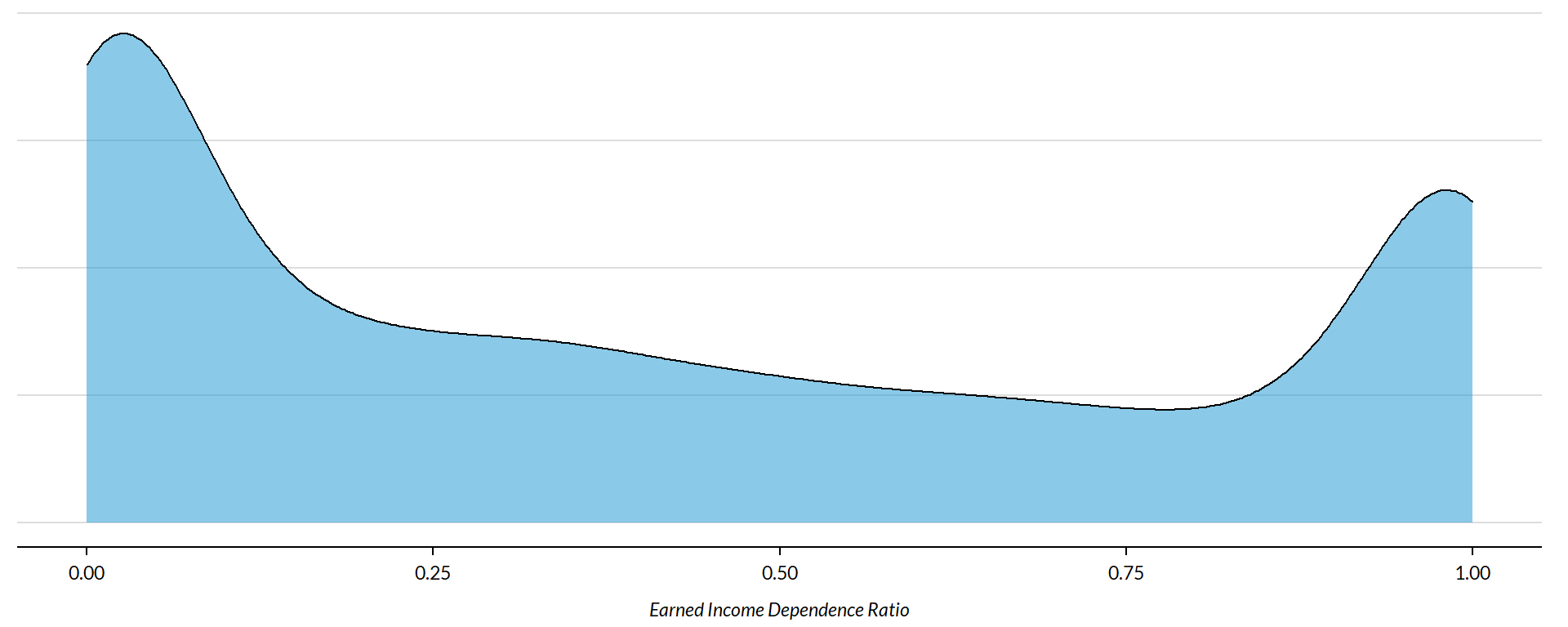

Earned Income Dependence Ratio by NTEE Major Code

core3 <- core2 %>% filter( ! is.na(NTEE1) )
table( core3$NTEE1) %>% sort(decreasing=TRUE) %>% kable()

Var1	Freq
Housing	2837
Community Development	1585
Human Services	1102


t <- table( factor(core3$NTEE1) ) 
df <- data.frame( x=Inf, y=Inf, 
                  N=paste0( "N=", as.character(t) ), 
                  NTEE1=names(t) )

ggplot( core3, aes( x=earned_income_ratio ) ) + 
  geom_density( alpha = 0.5) + 
  # xlim( -0.1, 1 ) +
  labs( title="Nonprofit Subsectors" ) + 
  xlab( variable.label2 ) + 
  facet_wrap( ~ NTEE1, nrow=1 ) + 
    theme_minimal( base_size = 15 )  + 
    theme( axis.title.y=element_blank(),
           axis.text.y=element_blank(), 
           axis.ticks.y=element_blank(),
           strip.text = element_text( face="bold") ) +  # size=20 
  geom_text( data=df, 
             aes(x, y, label=N ), 
             hjust=2, vjust=3, 
             color="gray60", size=6 )

Earned Income Dependence Ratio by Region

table( core2$Region) %>% kable()

Var1	Freq
Midwest	1444
Northeast	1368
South	1610
West	1088

t <- table( factor(core2$Region) ) 
df <- data.frame( x=Inf, y=Inf, 
                  N=paste0( "N=", as.character(t) ), 
                  Region=names(t) )

core2 %>% 
  filter( ! is.na(Region) ) %>% 
  ggplot( aes(earned_income_ratio) )  + 
    geom_density( alpha = 0.5 ) + 
    xlab( "Census Regions" ) + 
    ylab( variable.label2 ) +
    facet_wrap( ~ Region, nrow=3 ) + 
    theme_minimal( base_size = 22 )  + 
    theme( axis.title.y=element_blank(),
           axis.text.y=element_blank(), 
           axis.ticks.y=element_blank() ) + 
    geom_text( data=df, 
             aes(x, y, label=N ), 
             hjust=2, vjust=3, 
             color="gray60", size=6 )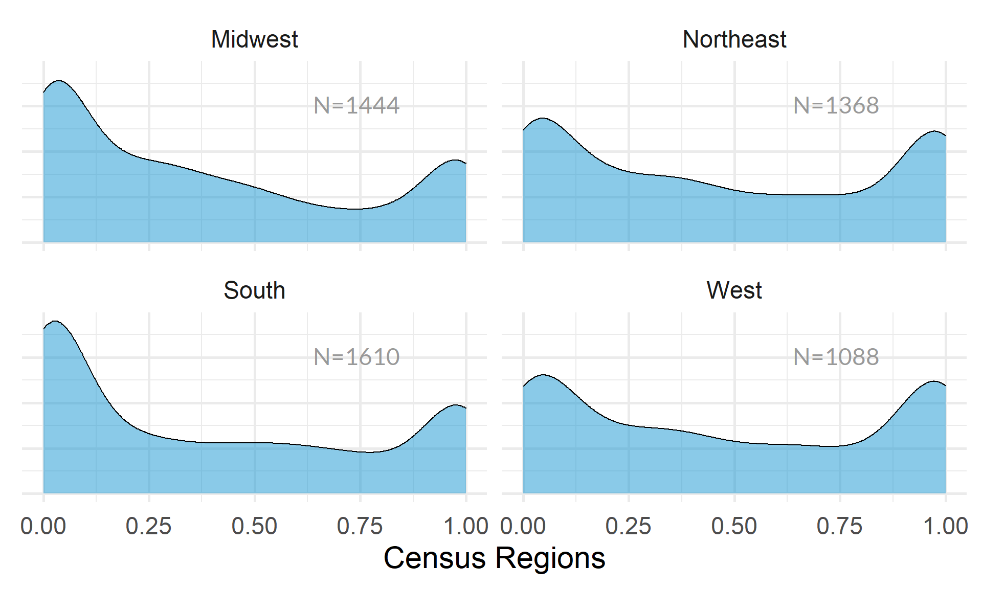

table( core2$Division ) %>% kable()

Var1	Freq
East North Central	1038
East South Central	289
Middle Atlantic	904
Mountain	303
New England	464
Pacific	785
South Atlantic	900
West North Central	406
West South Central	421

t <- table( factor(core2$Division) ) 
df <- data.frame( x=Inf, y=Inf, 
                  N=paste0( "N=", as.character(t) ), 
                  Division=names(t) )

core2 %>% 
  filter( ! is.na(Division) ) %>% 
  ggplot( aes(earned_income_ratio) )  + 
    geom_density( alpha = 0.5 ) + 
    xlab( "Census Sub-Regions (10)" ) + 
    ylab( variable.label2 ) +
    facet_wrap( ~ Division, nrow=3 ) + 
    theme_minimal( base_size = 22 )  + 
    theme( axis.title.y=element_blank(),
           axis.text.y=element_blank(), 
           axis.ticks.y=element_blank() ) + 
    geom_text( data=df, 
             aes(x, y, label=N ), 
             hjust=2, vjust=3, 
             color="gray60", size=6 )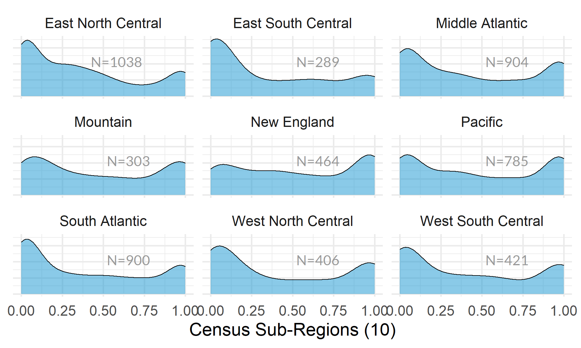

Earned Income Dependence Ratio by Nonprofit Size (Expenses)

ggplot( core2, aes(x = totfuncexpns )) +  
  geom_density( alpha = 0.5 ) + 
  xlim( quantile(core2$totfuncexpns, c(0.02,0.98), na.rm=T ) )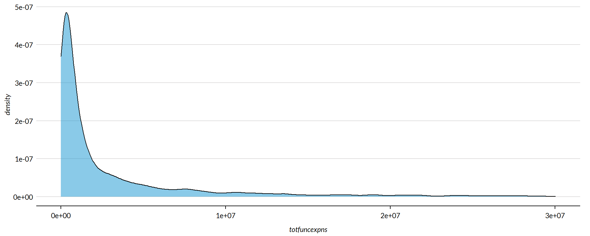

core2$totfuncexpns[ core2$totfuncexpns < 1 ] <- 1
# core2$totfuncexpns[ is.na(core2$totfuncexpns) ] <- 1

if( nrow(core2) > 10000 )
{
  core3 <- sample_n( core2, 10000 )
} else
{
  core3 <- core2
}

jplot( log10(core3$totfuncexpns), core3$earned_income_ratio, 
       xlab="Nonprofit Size (logged Expenses)", 
       ylab=variable.label2,
       xaxt="n", xlim=c(3,10) )
axis( side=1, 
      at=c(3,4,5,6,7,8,9,10), 
      labels=c("1k","10k","100k","1m","10m","100m","1b","10b") )

core2 %>% 
  filter( ! is.na(exp.q) ) %>% 
  ggplot( aes(earned_income_ratio) )  + 
    geom_density( alpha = 0.5) + 
    labs( title="Nonprofit Size (logged expenses)" ) + 
    xlab( variable.label2 ) +
    facet_wrap( ~ exp.q, nrow=3 ) + 
    theme_minimal( base_size = 22 )  + 
    theme( axis.title.y=element_blank(),
           axis.text.y=element_blank(), 
           axis.ticks.y=element_blank() )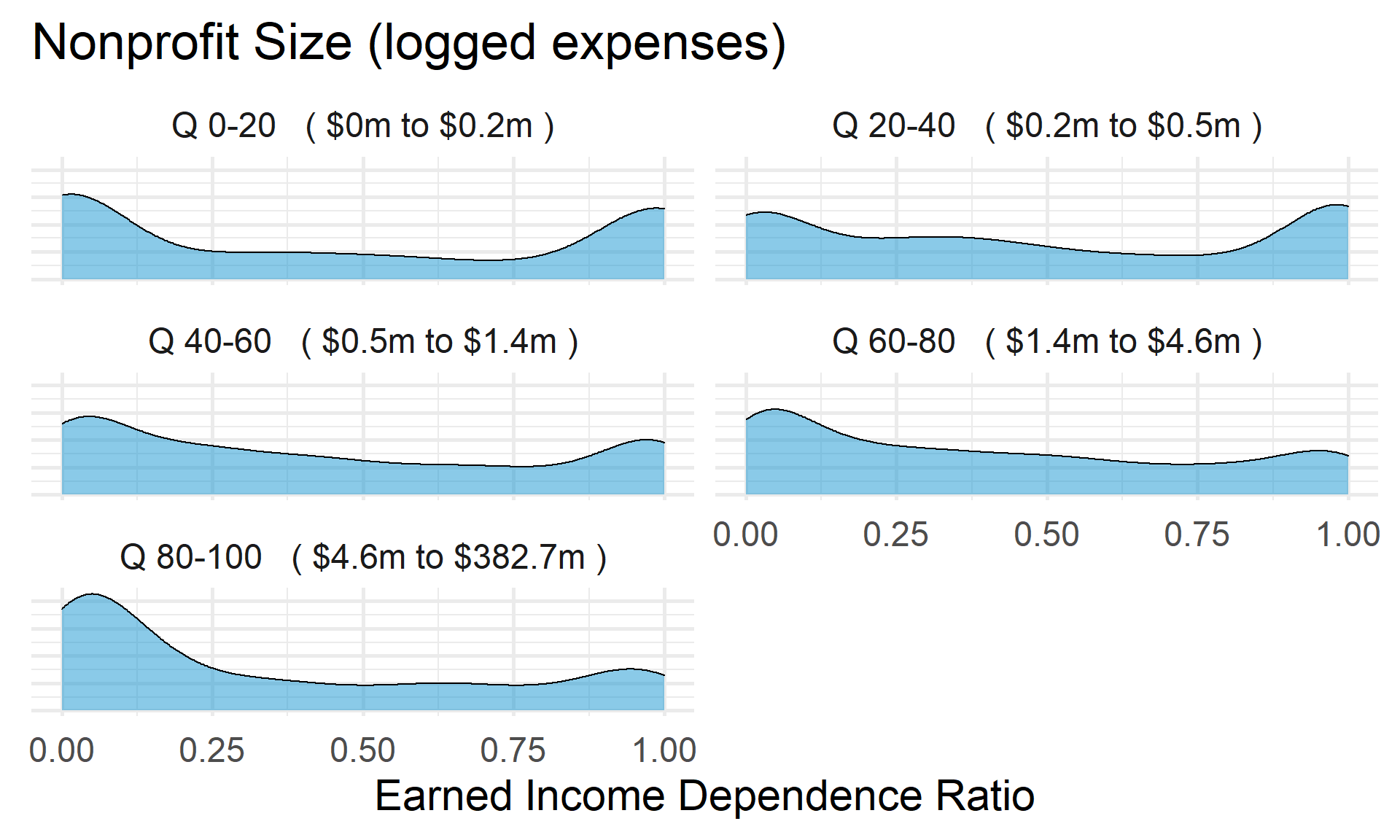

Earned Income Dependence Ratio by Nonprofit Size (Revenue)

ggplot( core2, aes(x = totrevenue )) +  
  geom_density( alpha = 0.5 ) + 
  xlim( quantile(core2$totrevenue, c(0.02,0.98), na.rm=T ) ) + 
  theme( axis.title.y=element_blank(),
           axis.text.y=element_blank(), 
           axis.ticks.y=element_blank() )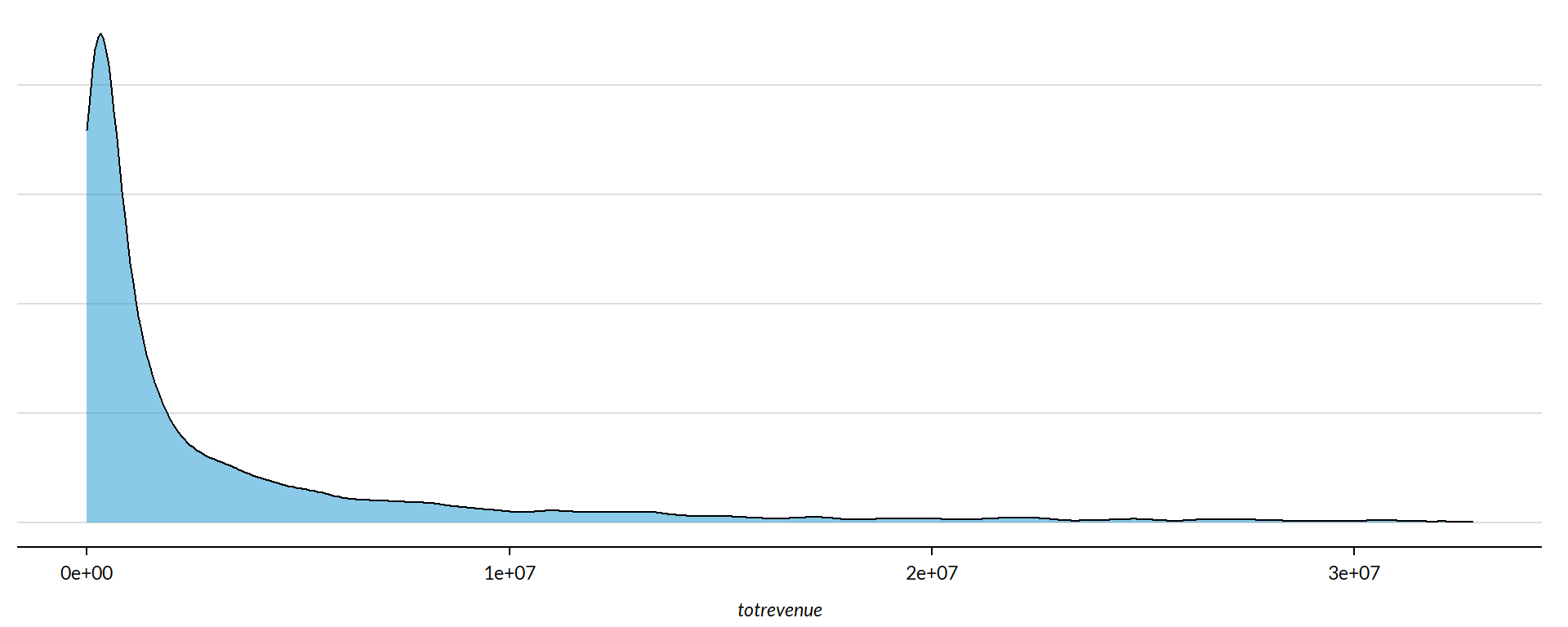

core2$totrevenue[ core2$totrevenue < 1 ] <- 1

if( nrow(core2) > 10000 )
{
  core3 <- sample_n( core2, 10000 )
} else
{
  core3 <- core2
}

jplot( log10(core3$totrevenue), core3$earned_income_ratio, 
       xlab="Nonprofit Size (logged Revenue)", 
       ylab=variable.label2,
       xaxt="n", xlim=c(3,10) )
axis( side=1, 
      at=c(3,4,5,6,7,8,9,10), 
      labels=c("1k","10k","100k","1m","10m","100m","1b","10b") )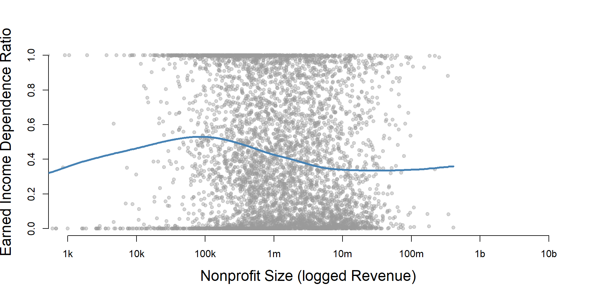

core2 %>% 
  filter( ! is.na(rev.q) ) %>% 
  ggplot( aes(earned_income_ratio) )  + 
    geom_density( alpha = 0.5 ) + 
    labs( title="Nonprofit Size (logged revenues)" ) + 
    xlab( variable.label2 ) +
    facet_wrap( ~ rev.q, nrow=3 ) + 
    theme_minimal( base_size = 22 )  + 
    theme( axis.title.y=element_blank(),
           axis.text.y=element_blank(), 
           axis.ticks.y=element_blank() )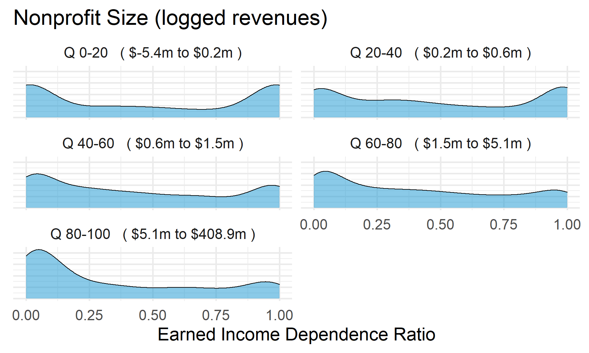

Earned Income Dependence Ratio by Nonprofit Size (Net Assets)

ggplot( core2, aes(x = totnetassetend )) +  
  geom_density( alpha = 0.5) + 
  xlim( quantile(core2$totnetassetend, c(0.02,0.98), na.rm=T ) ) + 
  xlab( "Net Assets" ) +
    theme( axis.title.y=element_blank(),
           axis.text.y=element_blank(), 
           axis.ticks.y=element_blank() )

core2$totnetassetend[ core2$totnetassetend < 1 ] <- NA

if( nrow(core2) > 10000 )
{
  core3 <- sample_n( core2, 10000 )
} else
{
  core3 <- core2
}

jplot( log10(core3$totnetassetend), core3$earned_income_ratio, 
       xlab="Nonprofit Size (logged Net Assets)", 
       ylab=variable.label2,
       xaxt="n", xlim=c(3,10) )
axis( side=1, 
      at=c(3,4,5,6,7,8,9,10), 
      labels=c("1k","10k","100k","1m","10m","100m","1b","10b") )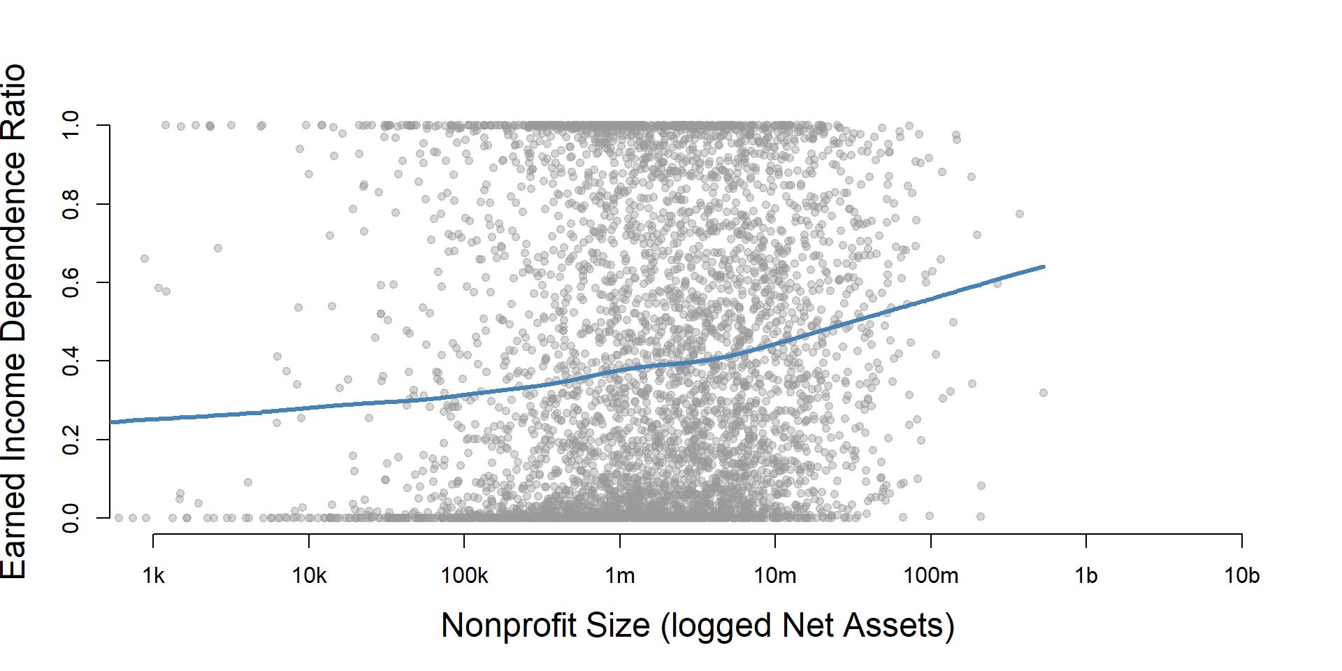

core2$totnetassetend[ core2$totnetassetend < 1 ] <- NA
core2$asset.q <- create_quantiles( var=core2$totnetassetend, n.groups=5 )

core2 %>% 
  filter( ! is.na(asset.q) ) %>% 
  ggplot( aes(earned_income_ratio) )  + 
    geom_density( alpha = 0.5 ) + 
    labs( title="Nonprofit Size (logged net assets, if assets > 0)" ) + 
    xlab( variable.label2 ) + 
    ylab( "" ) + 
    facet_wrap( ~ asset.q, nrow=3 ) + 
    theme_minimal( base_size = 22 )  + 
    theme( axis.title.y=element_blank(),
           axis.text.y=element_blank(), 
           axis.ticks.y=element_blank() )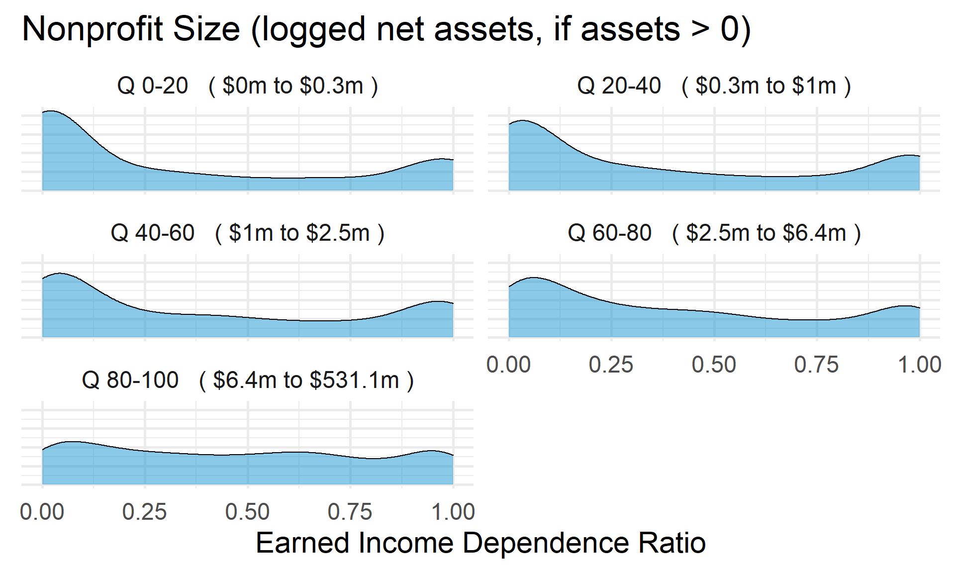

Total Assets for Comparison

core2$totassetsend[ core2$totassetsend < 1 ] <- NA
core2$tot.asset.q <- create_quantiles( var=core2$totassetsend, n.groups=5 )

if( nrow(core2) > 10000 )
{
  core3 <- sample_n( core2, 10000 )
} else
{
  core3 <- core2
}

jplot( log10(core3$totassetsend), core3$earned_income_ratio, 
       xlab="Nonprofit Size (logged Total Assets)", 
       ylab=variable.label2,
       xaxt="n", xlim=c(3,10) )
axis( side=1, 
      at=c(3,4,5,6,7,8,9,10), 
      labels=c("1k","10k","100k","1m","10m","100m","1b","10b") )

ggplot( core2, aes(x = totassetsend )) +  
  geom_density( alpha = 0.5) + 
  xlim( quantile(core2$totassetsend, c(0.02,0.98), na.rm=T ) ) + 
  xlab( "Net Assets" ) +
    theme( axis.title.y=element_blank(),
           axis.text.y=element_blank(), 
           axis.ticks.y=element_blank() )

core2 %>% 
  filter( ! is.na(tot.asset.q) ) %>% 
  ggplot( aes(earned_income_ratio) )  + 
    geom_density( alpha = 0.5 ) + 
    xlab( "Nonprofit Size (logged total assets, if assets > 0)" ) + 
    ylab( variable.label2 ) +
    facet_wrap( ~ tot.asset.q, nrow=3 ) + 
    theme_minimal( base_size = 22 )  + 
    theme( axis.title.y=element_blank(),
           axis.text.y=element_blank(), 
           axis.ticks.y=element_blank() )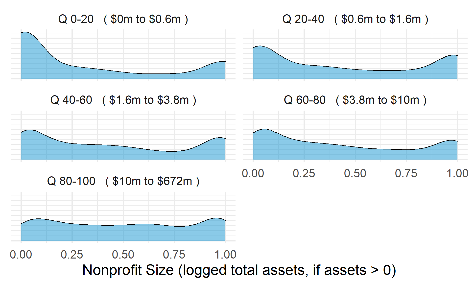

Earned Income Dependence Ratio by Nonprofit Age

ggplot( core2, aes(x = AGE )) +  
  geom_density( alpha = 0.5 )

core2$AGE[ core2$AGE < 1 ] <- NA

if( nrow(core2) > 10000 )
{
  core3 <- sample_n( core2, 10000 )
} else
{
  core3 <- core2
}

jplot( core3$AGE, core3$earned_income_ratio, 
       xlab="Nonprofit Age", 
       ylab=variable.label2 )

core2 %>% 
  filter( ! is.na(age.q) ) %>% 
  ggplot( aes(earned_income_ratio) )  + 
    geom_density( alpha = 0.5 ) + 
    labs( title="Nonprofit Age" ) + 
    xlab( variable.label2 ) +
    ylab( "" ) +
    facet_wrap( ~ age.q, nrow=3 ) + 
    theme_minimal( base_size = 22 )  + 
    theme( axis.title.y=element_blank(),
           axis.text.y=element_blank(), 
           axis.ticks.y=element_blank() )

Earned Income Dependence Ratio by Land and Building Value

ggplot( core2, aes(x = lndbldgsequipend )) +  
  geom_density( alpha = 0.5 )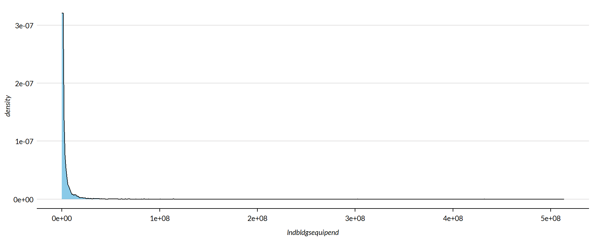

core2$lndbldgsequipend[ core2$lndbldgsequipend < 1 ] <- NA
if( nrow(core2) > 10000 )
{
  core3 <- sample_n( core2, 10000 )
} else
{
  core3 <- core2


jplot( log10(core3$lndbldgsequipend), core3$earned_income_ratio, 
       xlab="Land and Building Value (logged)", 
       ylab=variable.label2,
       xaxt="n", xlim=c(3,10) )
axis( side=1, 
      at=c(3,4,5,6,7,8,9,10), 
      labels=c("1k","10k","100k","1m","10m","100m","1b","10b") )
}

core2 %>% 
  filter( ! is.na(land.q) ) %>% 
  ggplot( aes(earned_income_ratio) )  + 
    geom_density( alpha = 0.5 ) + 
    labs( title="Land and Building Value" ) + 
    xlab( variable.label2 ) +
    ylab( "" ) +
    facet_wrap( ~ land.q, nrow=3 ) + 
    theme_minimal( base_size = 22 )  + 
    theme( axis.title.y=element_blank(),
           axis.text.y=element_blank(), 
           axis.ticks.y=element_blank() )

Investment Income Reliance Ratio Analysis

# TEMPORARY VARIABLES 
investment_income  <- core$invstmntinc + core$txexmptbndsproceeds + core$netrntlinc + core$netgnls
totalrevenues <- ( core$totrevenue )

# can't divide by zero
totalrevenues[ totalrevenues == 0 ] <- NA

# SAVE RESULTS 
core$investment_income_ratio <-  investment_income / totalrevenues
                     
# summary( core$investment_income_ratio )

Standardize Scales

Check high and low values to see what makes sense.

x.05 <- quantile( core$investment_income_ratio, 0.05, na.rm=T )
x.95 <- quantile( core$investment_income_ratio, 0.95, na.rm=T )

ggplot( core, aes(x = investment_income_ratio ) ) +  
  geom_density( alpha = 0.5) + 
  xlim( x.05, x.95 )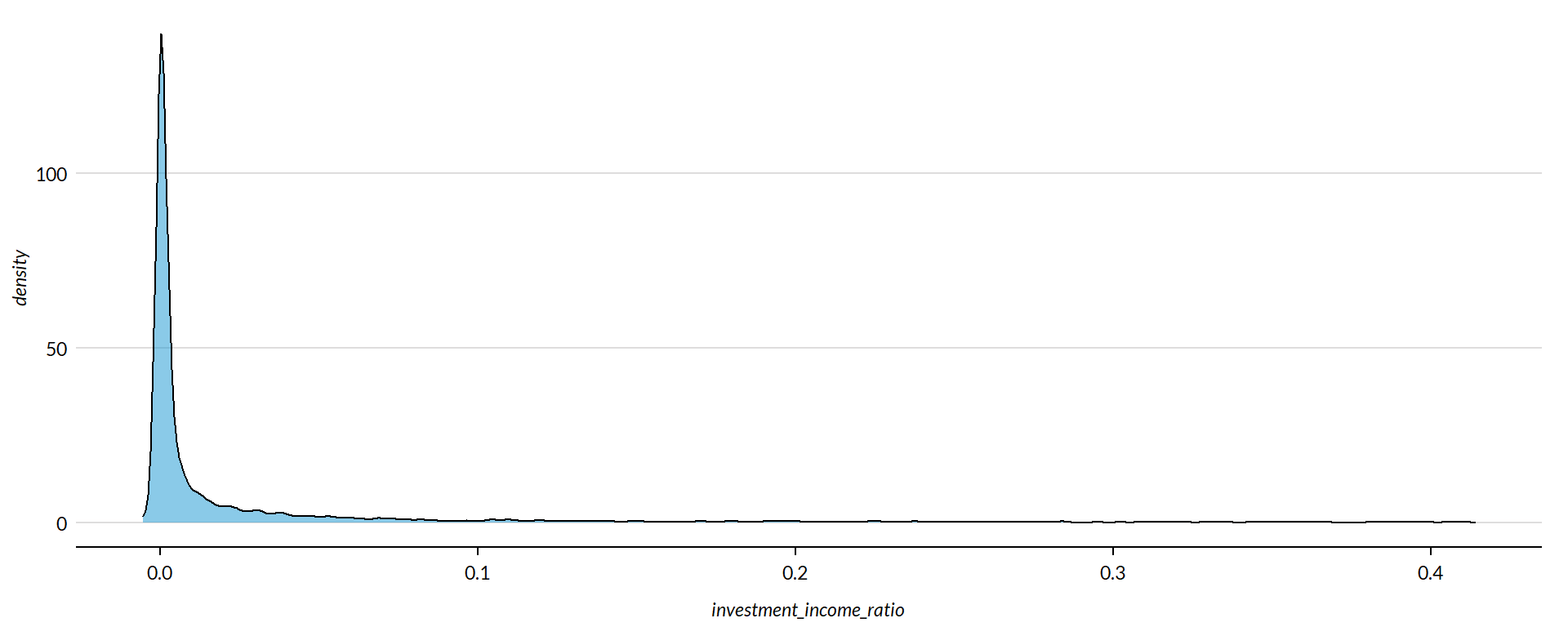

core2 <- core

# proportion of values that are negative
#mean( core2$investment_income_ratio < 0, na.rm=T ) 
#core2$investment_income_ratio[ core2$investment_income_ratio < 0 ] <- 0

# proption of values above 200% 
#mean( core2$investment_income_ratio > 50, na.rm=T ) 
#core2$investment_income_ratio[ core2$investment_income_ratio > 50 ] <- 50



x.05 <- quantile( core$investment_income_ratio, 0.05, na.rm=T )
x.95 <- quantile( core$investment_income_ratio, 0.95, na.rm=T )

core2 <- core

# proportion of values that are negative
# mean( core2$der < 0, na.rm=T ) 

# proption of values above 1% 
# mean( core2$der > 5, na.rm=T ) 

# WINSORIZATION AT 5th and 95th PERCENTILES

core2$investment_income_ratio[ core2$investment_income_ratio < x.05 ] <- x.05
core2$investment_income_ratio[ core2$investment_income_ratio > x.95 ] <- x.95

Metric Scope

Descriptive Statistics

Note: All monetary variables have been converted to thousands of dollars.


core2 %>%
  mutate( # investment_income_ratio = investment_income_ratio * 10000,
    totrevenue = totrevenue / 1000,
    totfuncexpns = totfuncexpns / 1000, 
    lndbldgsequipend = lndbldgsequipend / 1000,
    totassetsend = totassetsend / 1000,
    totliabend = totliabend / 1000,
    totnetassetend = totnetassetend / 1000 ) %>% 
  select( STATE,  NTEE1, NTMAJ12, 
          investment_income_ratio, 
          AGE, 
          totrevenue, totfuncexpns, 
          lndbldgsequipend, totassetsend, 
          totnetassetend, totliabend ) %>%

  stargazer( type = s.type, 
             digits=2, 
             summary.stat = c("min","p25","median",
                              "mean","p75","max", "sd"),
             covariate.labels = c("Investment Income Reliance Ratio", "Age", 
                                  "Revenue ($1k)", "Expenses($1k)", 
                                  "Buildings ($1k)", "Total Assets ($1k)",
                                  "Net Assets ($1k)", "Liabiliies ($1k)"))


Statistic	Min	Pctl(25)	Median	Mean	Pctl(75)	Max	St. Dev.

Investment Income Reliance Ratio	-0.01	0.00	0.001	0.04	0.02	0.41	0.10
Age	3	22	30	32.04	41	95	14.75
Revenue (1k)	-5,376.77	258.90	909.40	4,521.71	3,672.25	408,932.00	14,285.64
Expenses(1k)	0.00	263.50	840.06	4,192.08	3,327.50	382,666.50	13,465.77
Buildings (1k)	-4.48	79.14	824.25	3,504.47	2,868.50	513,508.80	13,210.06
Total Assets (1k)	-7,552.11	777.90	2,446.11	9,261.85	7,477.25	672,021.00	27,038.89
Net Assets (1k)	-178,869.70	155.67	1,093.86	4,553.27	4,078.70	531,067.70	15,470.31
Liabiliies (1k)	-2,707.10	115.44	815.58	4,708.51	3,133.16	705,623.10	18,721.86

What proportion of orgs have Investment Income Reliance Ratios equal to zero?

prop.zero <- mean( core2$investment_income_ratio == 0, na.rm=T )

In the sample, 18 percent of the organizations have Investment Income Reliance Ratios equal to zero, meaning they have no earned income. These organizations are dropped from subsequent graphs to keep the visualizations clean. The interpretation of the graphics should be the distributions of Investment Income Reliance Ratios for organizations that have positive or negative values.

###
### ADD QUANTILES
###
###   function create_quantiles() defined in r-functions.R

core2$exp.q   <- create_quantiles( var=core2$totfuncexpns,   n.groups=5 )
core2$rev.q   <- create_quantiles( var=core2$totrevenue,     n.groups=5 )
core2$asset.q <- create_quantiles( var=core2$totnetassetend, n.groups=5 )
core2$age.q   <- create_quantiles( var=core2$AGE,            n.groups=5 )
core2$land.q   <- create_quantiles( var=core2$lndbldgsequipend,   n.groups=5 )

Investment Income Dependence Ratio Density

min.x <- min( core2$investment_income_ratio, na.rm=T )
max.x <- max( core2$investment_income_ratio, na.rm=T )

ggplot( core2, aes(x = investment_income_ratio )) +  
  geom_density( alpha = 0.5 ) + 
  xlim( min.x, max.x  ) +
  xlab( variable.label3 ) +
  theme( axis.title.y=element_blank(),
         axis.text.y=element_blank(), 
         axis.ticks.y=element_blank() )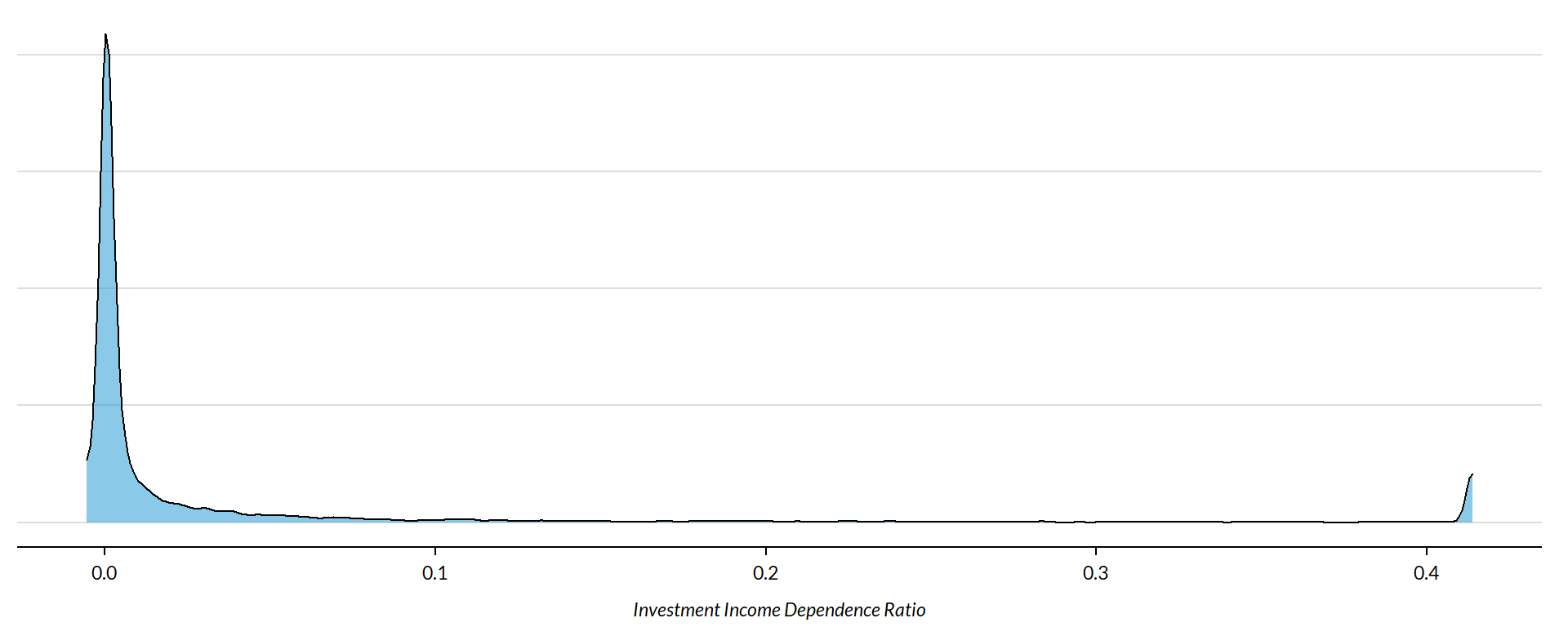

Investment Income Dependence Ratio by NTEE Major Code

core3 <- core2 %>% filter( ! is.na(NTEE1) )
table( core3$NTEE1) %>% sort(decreasing=TRUE) %>% kable()

Var1	Freq
Housing	2837
Community Development	1585
Human Services	1102


t <- table( factor(core3$NTEE1) ) 
df <- data.frame( x=Inf, y=Inf, 
                  N=paste0( "N=", as.character(t) ), 
                  NTEE1=names(t) )

ggplot( core3, aes( x=investment_income_ratio ) ) + 
  geom_density( alpha = 0.5) + 
  # xlim( -0.1, 1 ) +
  labs( title="Nonprofit Subsectors" ) + 
  xlab( variable.label3 ) + 
  facet_wrap( ~ NTEE1, nrow=1 ) + 
    theme_minimal( base_size = 15 )  + 
    theme( axis.title.y=element_blank(),
           axis.text.y=element_blank(), 
           axis.ticks.y=element_blank(),
           strip.text = element_text( face="bold") ) +  # size=20 
  geom_text( data=df, 
             aes(x, y, label=N ), 
             hjust=2, vjust=3, 
             color="gray60", size=6 )

Investment Income Dependence Ratio by Region

table( core2$Region) %>% kable()

Var1	Freq
Midwest	1444
Northeast	1368
South	1610
West	1088

t <- table( factor(core2$Region) ) 
df <- data.frame( x=Inf, y=Inf, 
                  N=paste0( "N=", as.character(t) ), 
                  Region=names(t) )

core2 %>% 
  filter( ! is.na(Region) ) %>% 
  ggplot( aes(investment_income_ratio) )  + 
    geom_density( alpha = 0.5 ) + 
    xlab( "Census Regions" ) + 
    ylab( variable.label3 ) +
    facet_wrap( ~ Region, nrow=3 ) + 
    theme_minimal( base_size = 22 )  + 
    theme( axis.title.y=element_blank(),
           axis.text.y=element_blank(), 
           axis.ticks.y=element_blank() ) + 
    geom_text( data=df, 
             aes(x, y, label=N ), 
             hjust=2, vjust=3, 
             color="gray60", size=6 )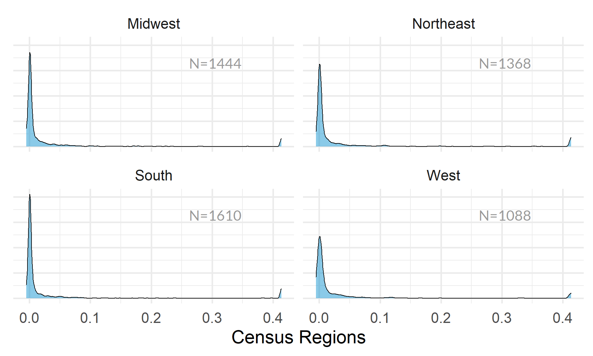

table( core2$Division ) %>% kable()

Var1	Freq
East North Central	1038
East South Central	289
Middle Atlantic	904
Mountain	303
New England	464
Pacific	785
South Atlantic	900
West North Central	406
West South Central	421

t <- table( factor(core2$Division) ) 
df <- data.frame( x=Inf, y=Inf, 
                  N=paste0( "N=", as.character(t) ), 
                  Division=names(t) )

core2 %>% 
  filter( ! is.na(Division) ) %>% 
  ggplot( aes(investment_income_ratio) )  + 
    geom_density( alpha = 0.5 ) + 
    xlab( "Census Sub-Regions (10)" ) + 
    ylab( variable.label3 ) +
    facet_wrap( ~ Division, nrow=3 ) + 
    theme_minimal( base_size = 22 )  + 
    theme( axis.title.y=element_blank(),
           axis.text.y=element_blank(), 
           axis.ticks.y=element_blank() ) + 
    geom_text( data=df, 
             aes(x, y, label=N ), 
             hjust=2, vjust=3, 
             color="gray60", size=6 )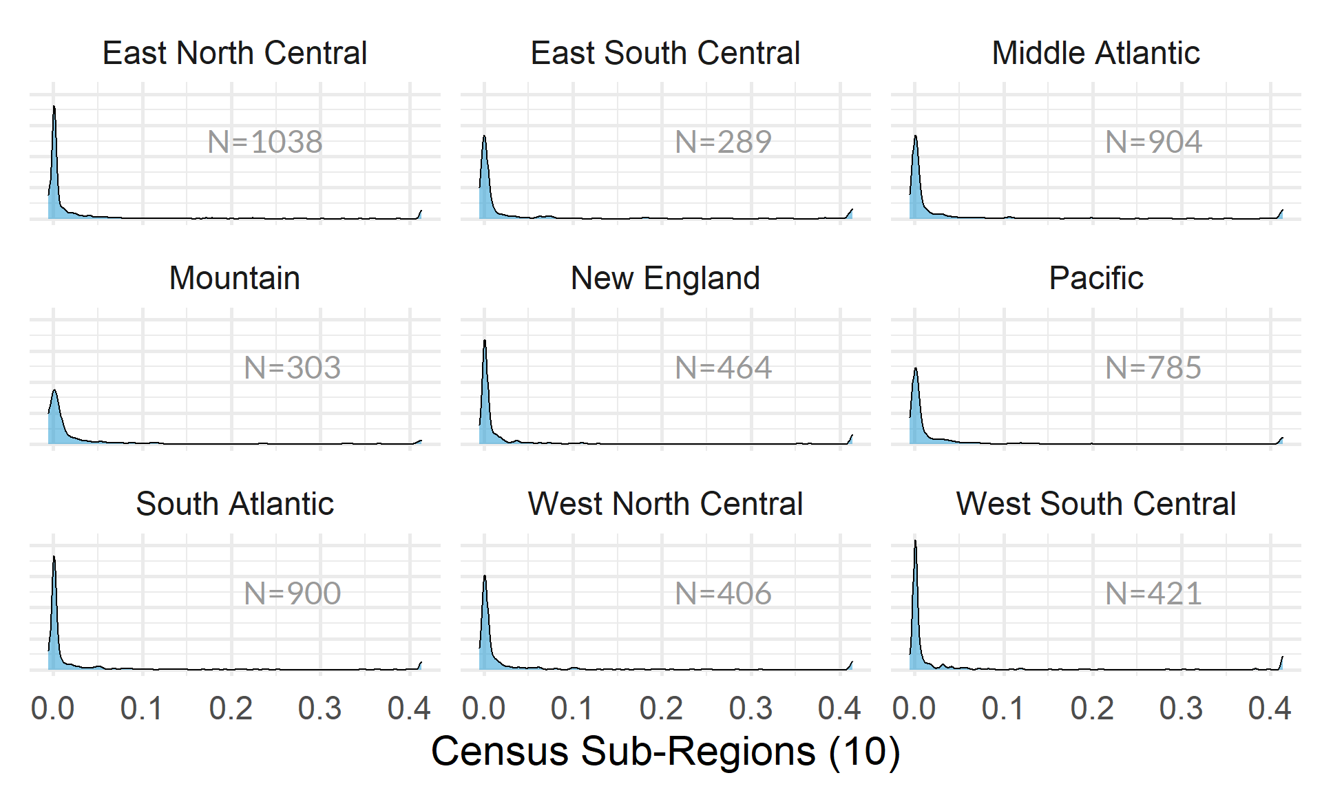

Investment Income Dependence Ratio by Nonprofit Size (Expenses)

ggplot( core2, aes(x = totfuncexpns )) +  
  geom_density( alpha = 0.5 ) + 
  xlim( quantile(core2$totfuncexpns, c(0.02,0.98), na.rm=T ) )

core2$totfuncexpns[ core2$totfuncexpns < 1 ] <- 1
# core2$totfuncexpns[ is.na(core2$totfuncexpns) ] <- 1

if( nrow(core2) > 10000 )
{
  core3 <- sample_n( core2, 10000 )
} else
{
  core3 <- core2
}

jplot( log10(core3$totfuncexpns), core3$investment_income_ratio, 
       xlab="Nonprofit Size (logged Expenses)", 
       ylab=variable.label3,
       xaxt="n", xlim=c(3,10) )
axis( side=1, 
      at=c(3,4,5,6,7,8,9,10), 
      labels=c("1k","10k","100k","1m","10m","100m","1b","10b") )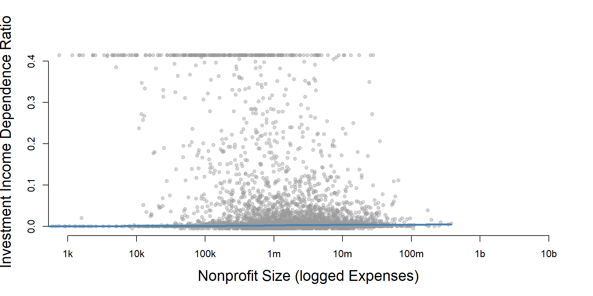

core2 %>% 
  filter( ! is.na(exp.q) ) %>% 
  ggplot( aes(investment_income_ratio) )  + 
    geom_density( alpha = 0.5) + 
    labs( title="Nonprofit Size (logged expenses)" ) + 
    xlab( variable.label3 ) +
    facet_wrap( ~ exp.q, nrow=3 ) + 
    theme_minimal( base_size = 22 )  + 
    theme( axis.title.y=element_blank(),
           axis.text.y=element_blank(), 
           axis.ticks.y=element_blank() )

Investment Income Dependence Ratio by Nonprofit Size (Revenue)

ggplot( core2, aes(x = totrevenue )) +  
  geom_density( alpha = 0.5 ) + 
  xlim( quantile(core2$totrevenue, c(0.02,0.98), na.rm=T ) ) + 
  theme( axis.title.y=element_blank(),
           axis.text.y=element_blank(), 
           axis.ticks.y=element_blank() )

core2$totrevenue[ core2$totrevenue < 1 ] <- 1

if( nrow(core2) > 10000 )
{
  core3 <- sample_n( core2, 10000 )
} else
{
  core3 <- core2
}

jplot( log10(core3$totrevenue), core3$investment_income_ratio, 
       xlab="Nonprofit Size (logged Revenue)", 
       ylab=variable.label3,
       xaxt="n", xlim=c(3,10) )
axis( side=1, 
      at=c(3,4,5,6,7,8,9,10), 
      labels=c("1k","10k","100k","1m","10m","100m","1b","10b") )

core2 %>% 
  filter( ! is.na(rev.q) ) %>% 
  ggplot( aes(investment_income_ratio) )  + 
    geom_density( alpha = 0.5 ) + 
    labs( title="Nonprofit Size (logged revenues)" ) + 
    xlab( variable.label3 ) +
    facet_wrap( ~ rev.q, nrow=3 ) + 
    theme_minimal( base_size = 22 )  + 
    theme( axis.title.y=element_blank(),
           axis.text.y=element_blank(), 
           axis.ticks.y=element_blank() )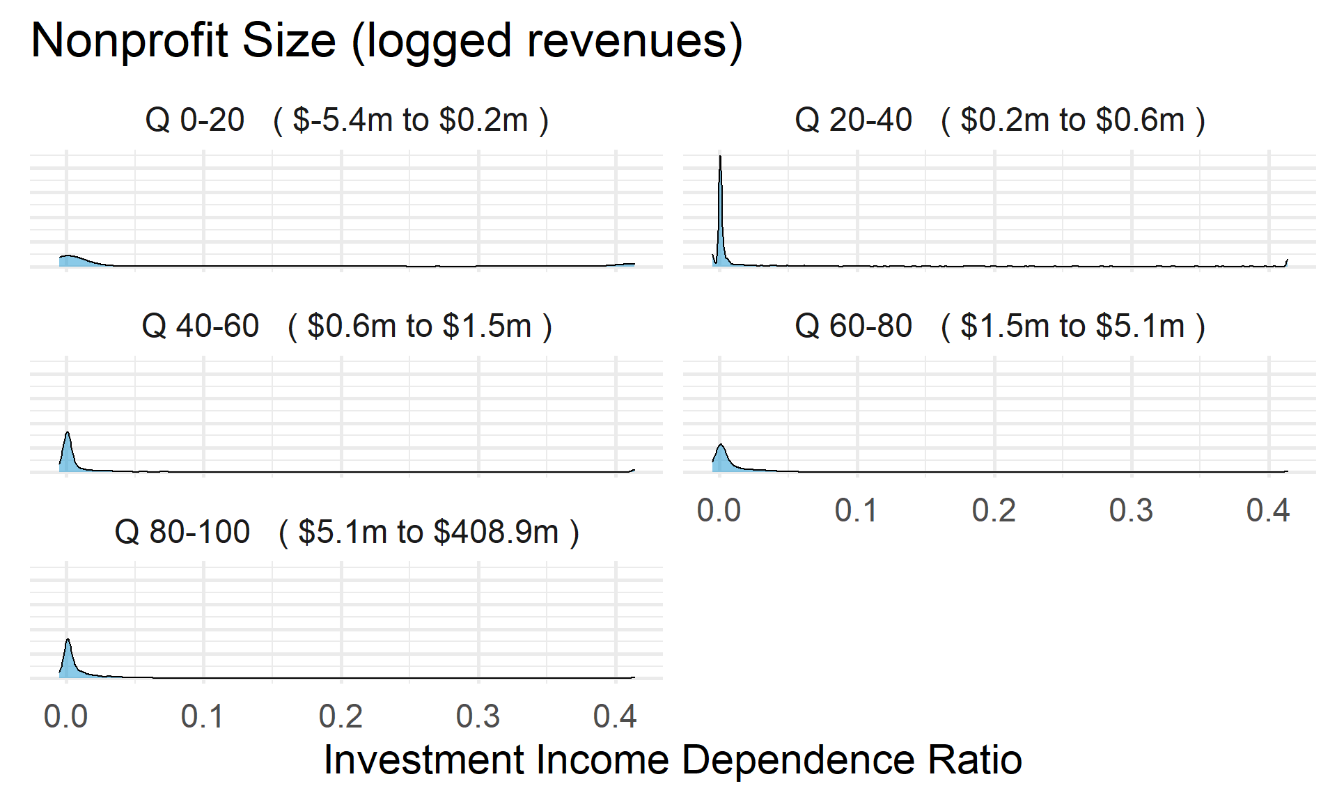

Investment Income Dependence Ratio by Nonprofit Size (Net Assets)

ggplot( core2, aes(x = totnetassetend )) +  
  geom_density( alpha = 0.5) + 
  xlim( quantile(core2$totnetassetend, c(0.02,0.98), na.rm=T ) ) + 
  xlab( "Net Assets" ) +
    theme( axis.title.y=element_blank(),
           axis.text.y=element_blank(), 
           axis.ticks.y=element_blank() )

core2$totnetassetend[ core2$totnetassetend < 1 ] <- NA

if( nrow(core2) > 10000 )
{
  core3 <- sample_n( core2, 10000 )
} else
{
  core3 <- core2
}

jplot( log10(core3$totnetassetend), core3$investment_income_ratio, 
       xlab="Nonprofit Size (logged Net Assets)", 
       ylab=variable.label3,
       xaxt="n", xlim=c(3,10) )
axis( side=1, 
      at=c(3,4,5,6,7,8,9,10), 
      labels=c("1k","10k","100k","1m","10m","100m","1b","10b") )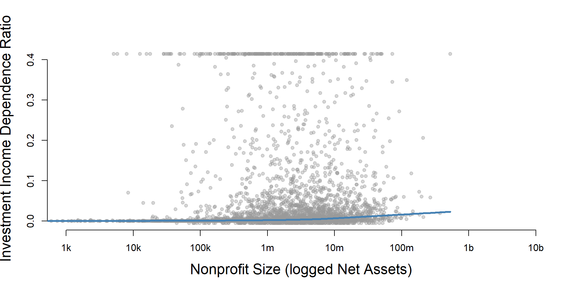

core2$totnetassetend[ core2$totnetassetend < 1 ] <- NA
core2$asset.q <- create_quantiles( var=core2$totnetassetend, n.groups=5 )

core2 %>% 
  filter( ! is.na(asset.q) ) %>% 
  ggplot( aes(investment_income_ratio) )  + 
    geom_density( alpha = 0.5 ) + 
    labs( title="Nonprofit Size (logged net assets, if assets > 0)" ) + 
    xlab( variable.label3 ) + 
    ylab( "" ) + 
    facet_wrap( ~ asset.q, nrow=3 ) + 
    theme_minimal( base_size = 22 )  + 
    theme( axis.title.y=element_blank(),
           axis.text.y=element_blank(), 
           axis.ticks.y=element_blank() )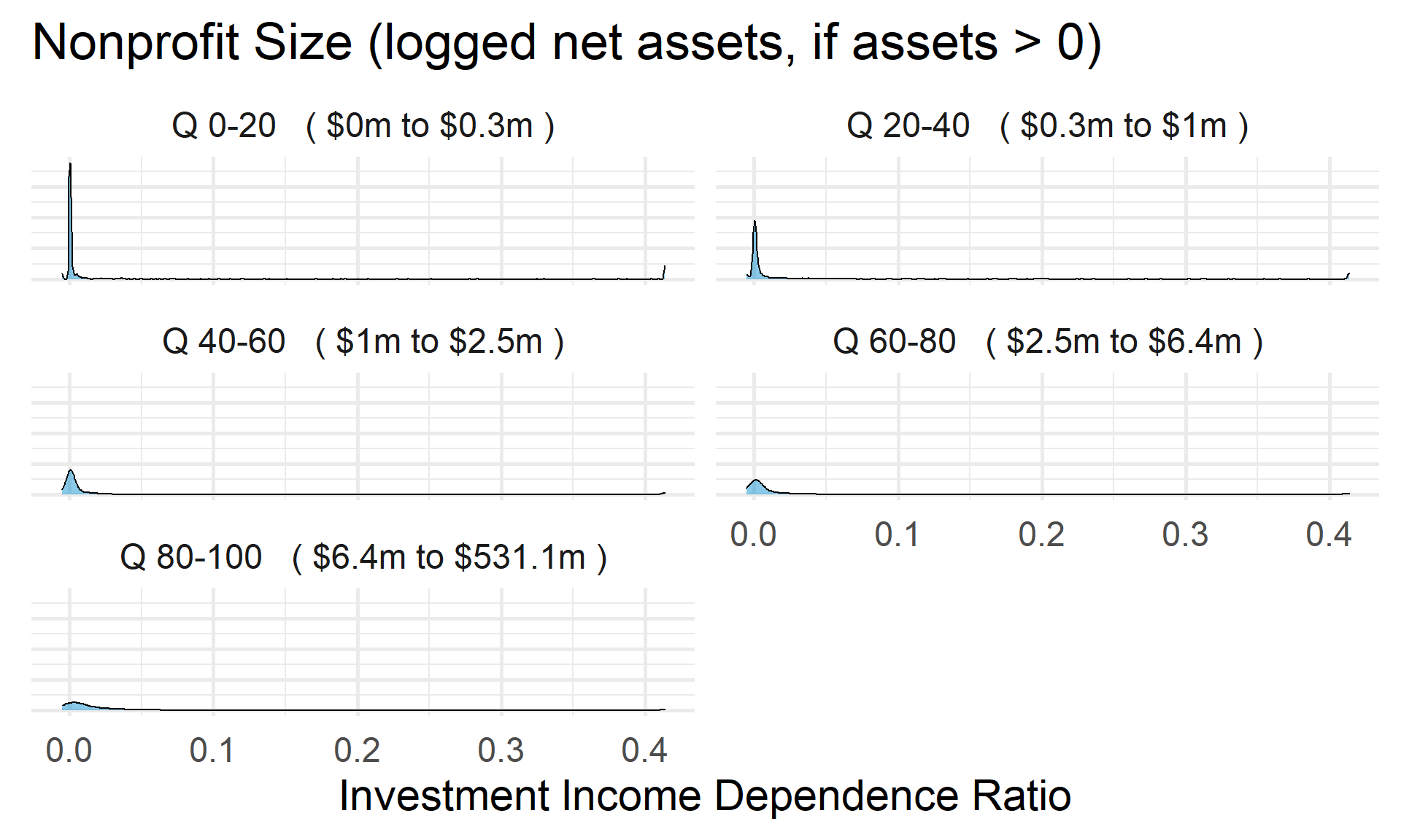

Total Assets for Comparison

core2$totassetsend[ core2$totassetsend < 1 ] <- NA
core2$tot.asset.q <- create_quantiles( var=core2$totassetsend, n.groups=5 )

if( nrow(core2) > 10000 )
{
  core3 <- sample_n( core2, 10000 )
} else
{
  core3 <- core2
}

jplot( log10(core3$totassetsend), core3$investment_income_ratio, 
       xlab="Nonprofit Size (logged Total Assets)", 
       ylab=variable.label3,
       xaxt="n", xlim=c(3,10) )
axis( side=1, 
      at=c(3,4,5,6,7,8,9,10), 
      labels=c("1k","10k","100k","1m","10m","100m","1b","10b") )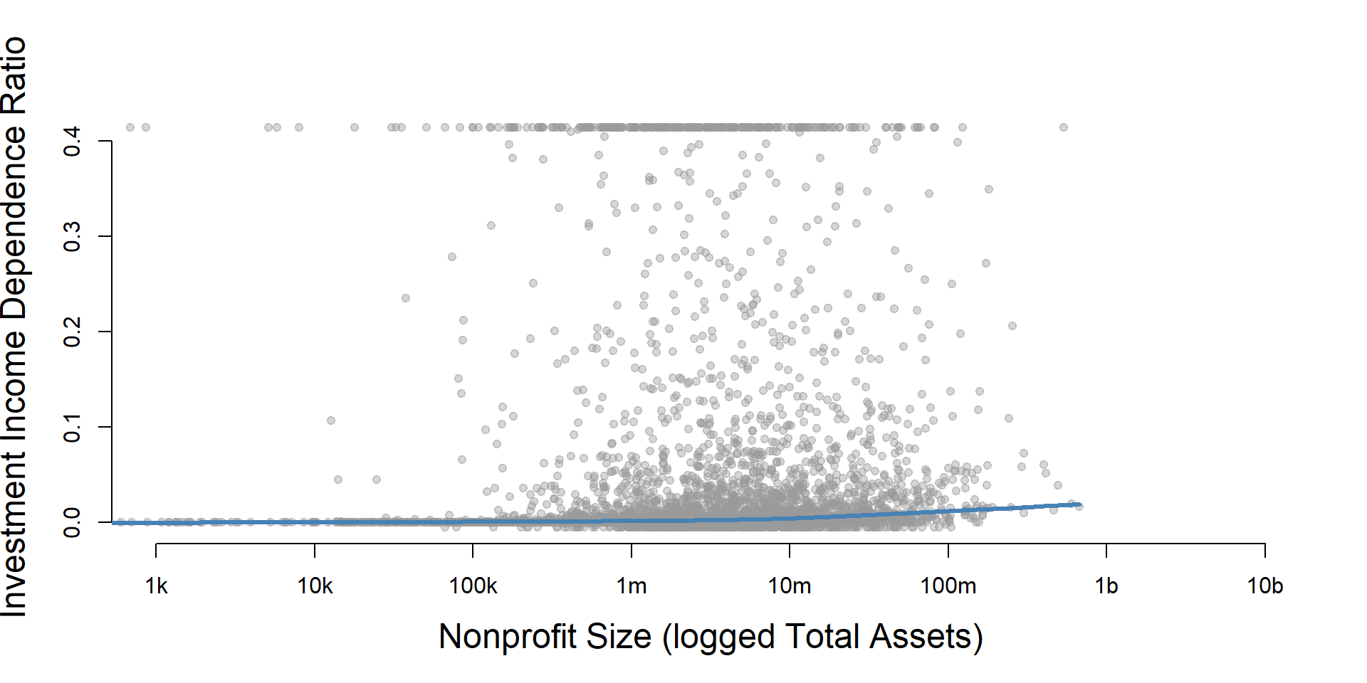

ggplot( core2, aes(x = totassetsend )) +  
  geom_density( alpha = 0.5) + 
  xlim( quantile(core2$totassetsend, c(0.02,0.98), na.rm=T ) ) + 
  xlab( "Net Assets" ) +
    theme( axis.title.y=element_blank(),
           axis.text.y=element_blank(), 
           axis.ticks.y=element_blank() )

core2 %>% 
  filter( ! is.na(tot.asset.q) ) %>% 
  ggplot( aes(investment_income_ratio) )  + 
    geom_density( alpha = 0.5 ) + 
    xlab( "Nonprofit Size (logged total assets, if assets > 0)" ) + 
    ylab( variable.label3 ) +
    facet_wrap( ~ tot.asset.q, nrow=3 ) + 
    theme_minimal( base_size = 22 )  + 
    theme( axis.title.y=element_blank(),
           axis.text.y=element_blank(), 
           axis.ticks.y=element_blank() )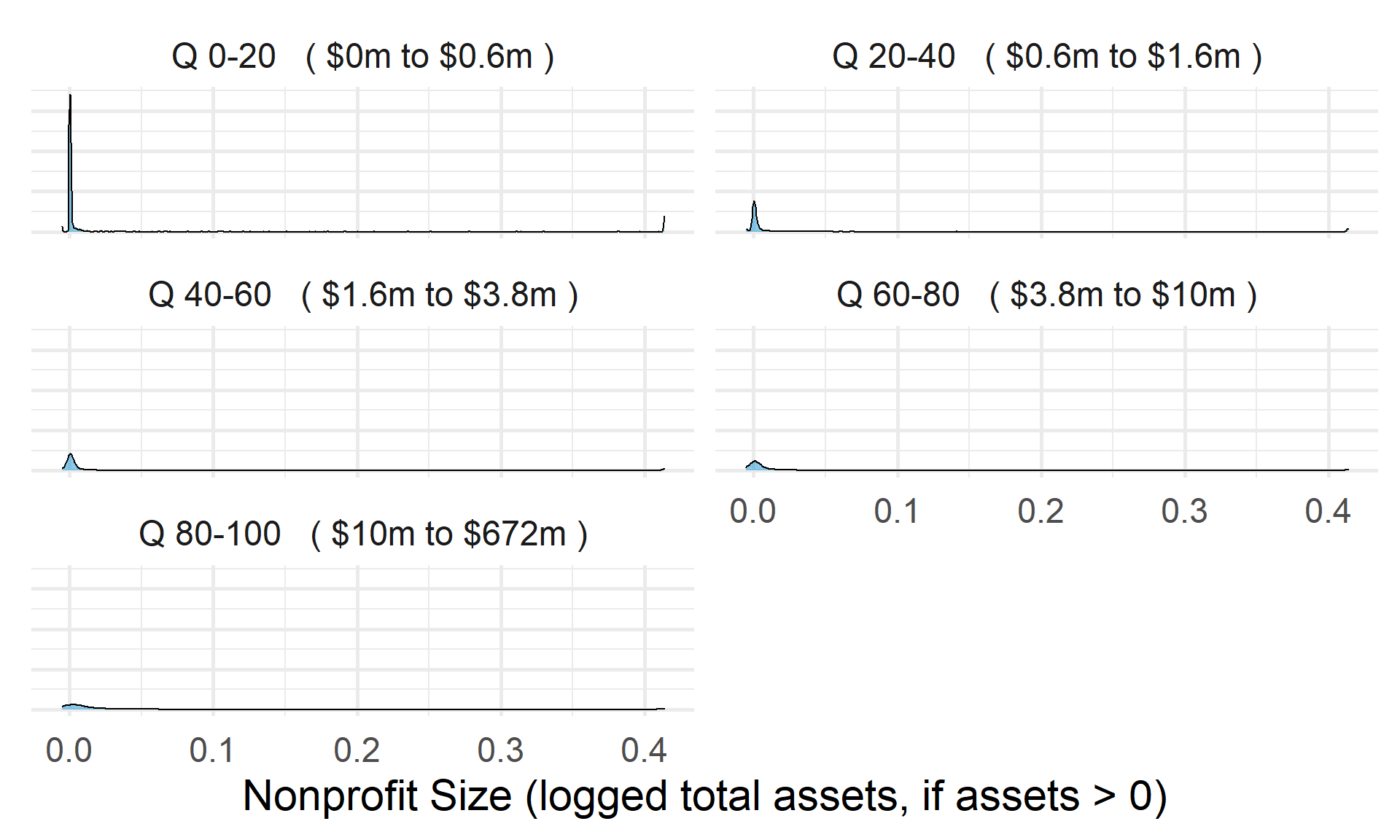

Investment Income Dependence Ratio by Nonprofit Age

ggplot( core2, aes(x = AGE )) +  
  geom_density( alpha = 0.5 )

core2$AGE[ core2$AGE < 1 ] <- NA

if( nrow(core2) > 10000 )
{
  core3 <- sample_n( core2, 10000 )
} else
{
  core3 <- core2
}

jplot( core3$AGE, core3$investment_income_ratio, 
       xlab="Nonprofit Age", 
       ylab=variable.label3 )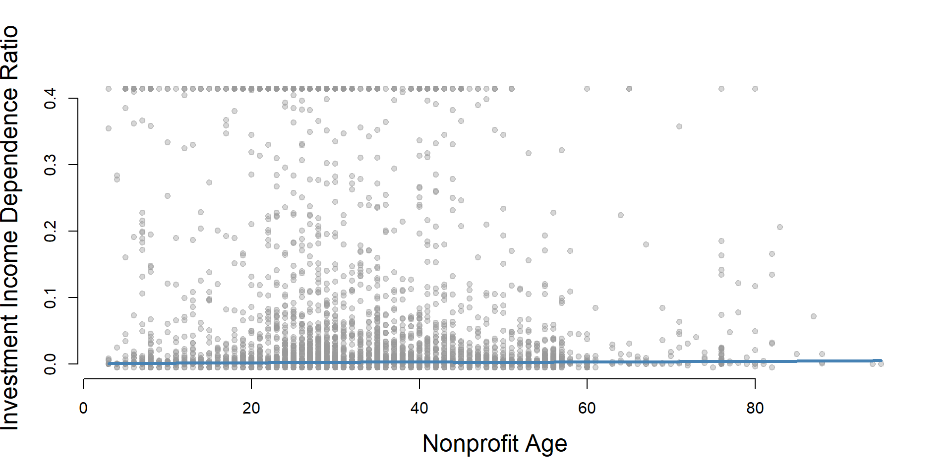

core2 %>% 
  filter( ! is.na(age.q) ) %>% 
  ggplot( aes(investment_income_ratio) )  + 
    geom_density( alpha = 0.5 ) + 
    labs( title="Nonprofit Age" ) + 
    xlab( variable.label3 ) +
    ylab( "" ) +
    facet_wrap( ~ age.q, nrow=3 ) + 
    theme_minimal( base_size = 22 )  + 
    theme( axis.title.y=element_blank(),
           axis.text.y=element_blank(), 
           axis.ticks.y=element_blank() )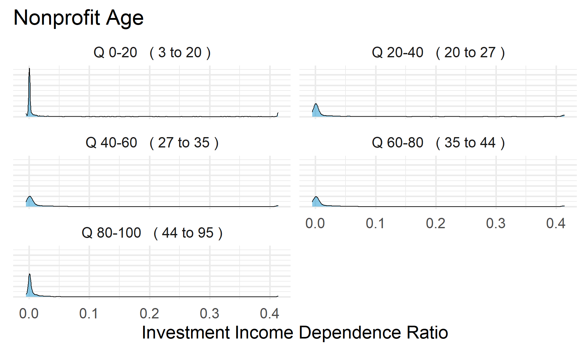

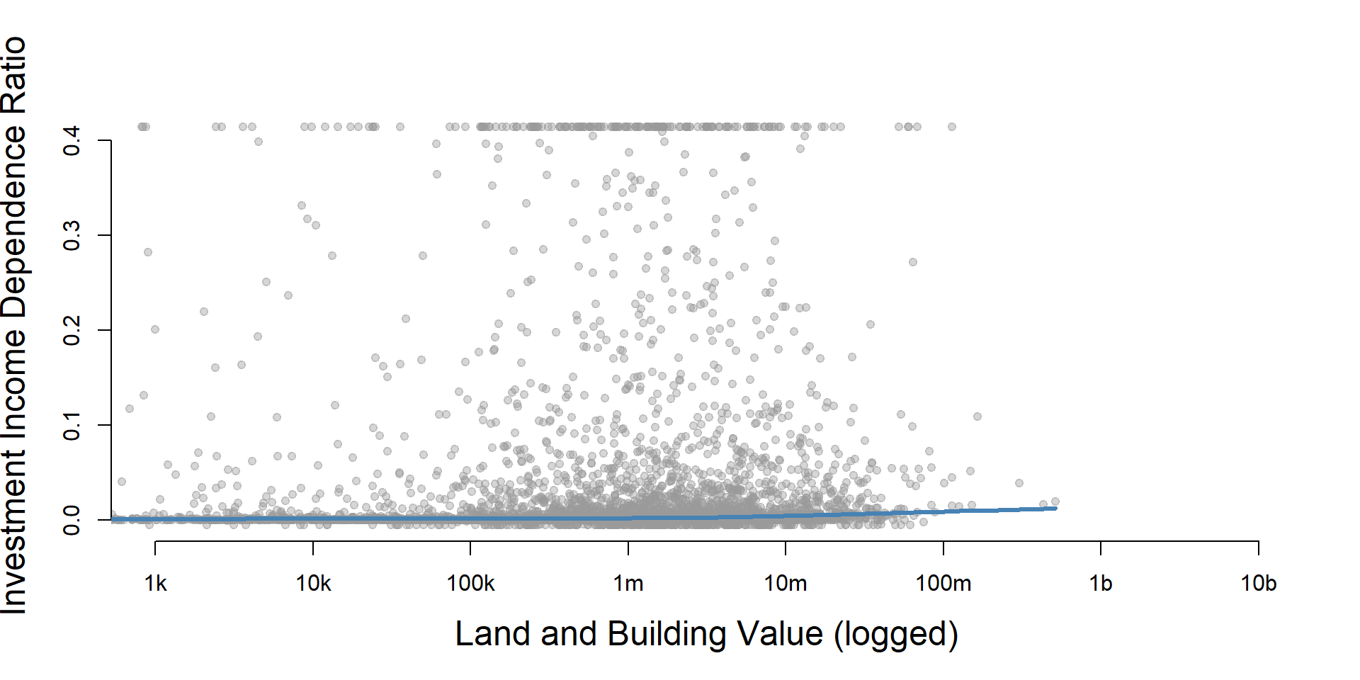
Investment Income Dependence Ratio by Land and Building Value

ggplot( core2, aes(x = lndbldgsequipend )) +  
  geom_density( alpha = 0.5 )

core2$lndbldgsequipend[ core2$lndbldgsequipend < 1 ] <- NA
if( nrow(core2) > 10000 )
{
  core3 <- sample_n( core2, 10000 )
} else
{
  core3 <- core2


jplot( log10(core3$lndbldgsequipend), core3$investment_income_ratio, 
       xlab="Land and Building Value (logged)", 
       ylab=variable.label3,
       xaxt="n", xlim=c(3,10) )
axis( side=1, 
      at=c(3,4,5,6,7,8,9,10), 
      labels=c("1k","10k","100k","1m","10m","100m","1b","10b") )
}

core2 %>% 
  filter( ! is.na(land.q) ) %>% 
  ggplot( aes(investment_income_ratio) )  + 
    geom_density( alpha = 0.5 ) + 
    labs( title="Land and Building Value" ) + 
    xlab( variable.label3 ) +
    ylab( "" ) +
    facet_wrap( ~ land.q, nrow=3 ) + 
    theme_minimal( base_size = 22 )  + 
    theme( axis.title.y=element_blank(),
           axis.text.y=element_blank(), 
           axis.ticks.y=element_blank() )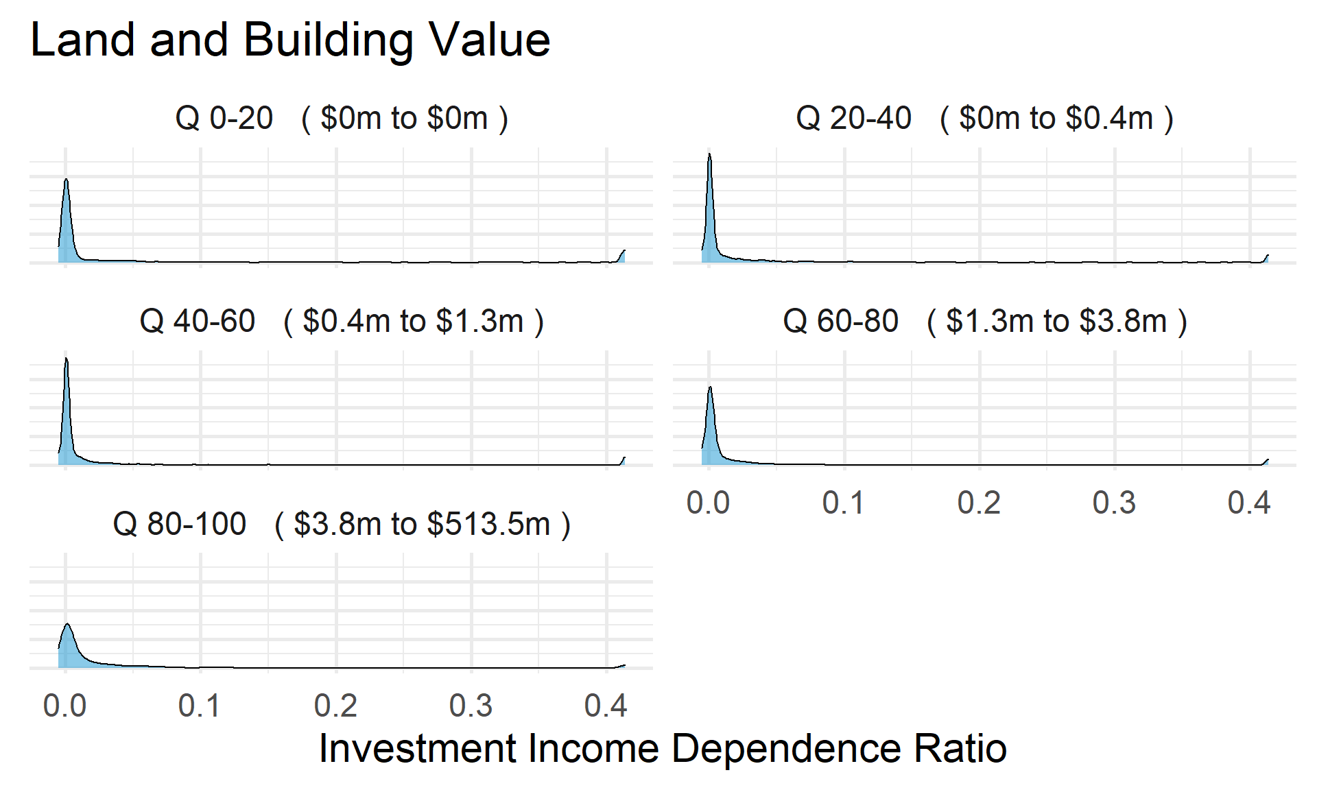

Income Reliance Ratio Analysis


dat <- dplyr::select(core3, donation_ratio, investment_income_ratio, earned_income_ratio )

core$income_reliance_ratio <- apply( dat, MARGIN=1, FUN=max )

                     
# summary( core3$income_reliance_ratio )

Standardize Scales

Check high and low values to see what makes sense.

x.05 <- quantile( core$income_reliance_ratio, 0.05, na.rm=T )
x.95 <- quantile( core$income_reliance_ratio, 0.95, na.rm=T )

ggplot( core, aes(x = income_reliance_ratio ) ) +  
  geom_density( alpha = 0.5) + 
  xlim( x.05, x.95 )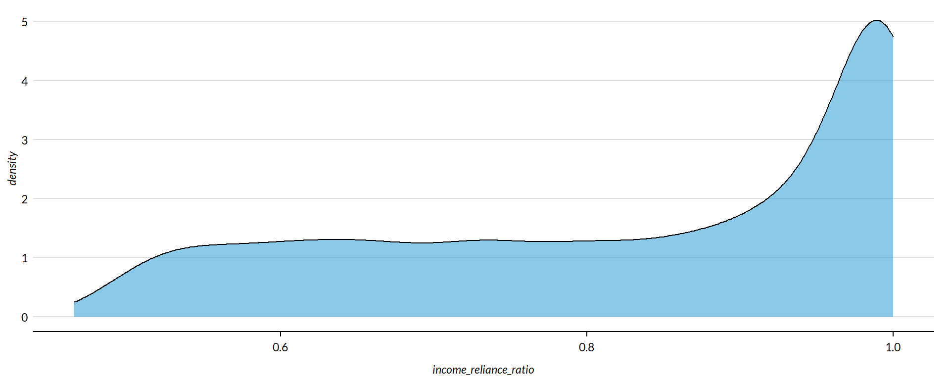

core2 <- core

# proportion of values that are negative
#mean( core3$income_reliance_ratio < 0, na.rm=T ) 
#core3$income_reliance_ratio[ core3$income_reliance_ratio < 0 ] <- 0

# proption of values above 200% 
#mean( core3$income_reliance_ratio > 50, na.rm=T ) 
#core3$income_reliance_ratio[ core3$income_reliance_ratio > 50 ] <- 50



x.05 <- quantile( core$income_reliance_ratio, 0.05, na.rm=T )
x.95 <- quantile( core$income_reliance_ratio, 0.95, na.rm=T )

core2 <- core

# proportion of values that are negative
# mean( core2$der < 0, na.rm=T ) 

# proption of values above 1% 
# mean( core2$der > 5, na.rm=T ) 

# WINSORIZATION AT 5th and 95th PERCENTILES

core2$income_reliance_ratio[ core2$income_reliance_ratio < x.05 ] <- x.05
core2$income_reliance_ratio[ core2$income_reliance_ratio > x.95 ] <- x.95

Metric Scope

Descriptive Statistics

Note: All monetary variables have been converted to thousands of dollars.


core2 %>%
  mutate( # income_reliance_ratio = income_reliance_ratio * 10000,
    totrevenue = totrevenue / 1000,
    totfuncexpns = totfuncexpns / 1000, 
    lndbldgsequipend = lndbldgsequipend / 1000,
    totassetsend = totassetsend / 1000,
    totliabend = totliabend / 1000,
    totnetassetend = totnetassetend / 1000 ) %>% 
  select( STATE,  NTEE1, NTMAJ12, 
          income_reliance_ratio, 
          AGE, 
          totrevenue, totfuncexpns, 
          lndbldgsequipend, totassetsend, 
          totnetassetend, totliabend ) %>%

  stargazer( type = s.type, 
             digits=2, 
             summary.stat = c("min","p25","median",
                              "mean","p75","max", "sd"),
             covariate.labels = c("Income  Reliance Ratio", "Age", 
                                  "Revenue ($1k)", "Expenses($1k)", 
                                  "Buildings ($1k)", "Total Assets ($1k)",
                                  "Net Assets ($1k)", "Liabiliies ($1k)"))


Statistic	Min	Pctl(25)	Median	Mean	Pctl(75)	Max	St. Dev.

Income Reliance Ratio	0.47	0.66	0.87	0.82	0.99	1.00	0.18
Age	3	22	30	32.04	41	95	14.75
Revenue (1k)	-5,376.77	258.90	909.40	4,521.71	3,672.25	408,932.00	14,285.64
Expenses(1k)	0.00	263.50	840.06	4,192.08	3,327.50	382,666.50	13,465.77
Buildings (1k)	-4.48	79.14	824.25	3,504.47	2,868.50	513,508.80	13,210.06
Total Assets (1k)	-7,552.11	777.90	2,446.11	9,261.85	7,477.25	672,021.00	27,038.89
Net Assets (1k)	-178,869.70	155.67	1,093.86	4,553.27	4,078.70	531,067.70	15,470.31
Liabiliies (1k)	-2,707.10	115.44	815.58	4,708.51	3,133.16	705,623.10	18,721.86

What proportion of orgs have Income Reliance Ratios equal to zero?

prop.zero <- mean( core$income_reliance_ratio == 0, na.rm=T )

In the sample, 0 percent of the organizations have Income Reliance Ratios equal to zero, meaning their highest source of income is equal to zero. These organizations are dropped from subsequent graphs to keep the visualizations clean. The interpretation of the graphics should be the distributions of Income Reliance Ratios for organizations that have positive or negative values.

###
### ADD QUANTILES
###
###   function create_quantiles() defined in r-functions.R

core2$exp.q   <- create_quantiles( var=core2$totfuncexpns,   n.groups=5 )
core2$rev.q   <- create_quantiles( var=core2$totrevenue,     n.groups=5 )
core2$asset.q <- create_quantiles( var=core2$totnetassetend, n.groups=5 )
core2$age.q   <- create_quantiles( var=core2$AGE,            n.groups=5 )
core2$land.q   <- create_quantiles( var=core2$lndbldgsequipend,   n.groups=5 )

Income Reliance Ratio Density

min.x <- min( core2$income_reliance_ratio, na.rm=T )
max.x <- max( core2$income_reliance_ratio, na.rm=T )

ggplot( core2, aes(x = income_reliance_ratio )) +  
  geom_density( alpha = 0.5 ) + 
  xlim( min.x, max.x  ) +
  xlab( variable.label4 ) +
  theme( axis.title.y=element_blank(),
         axis.text.y=element_blank(), 
         axis.ticks.y=element_blank() )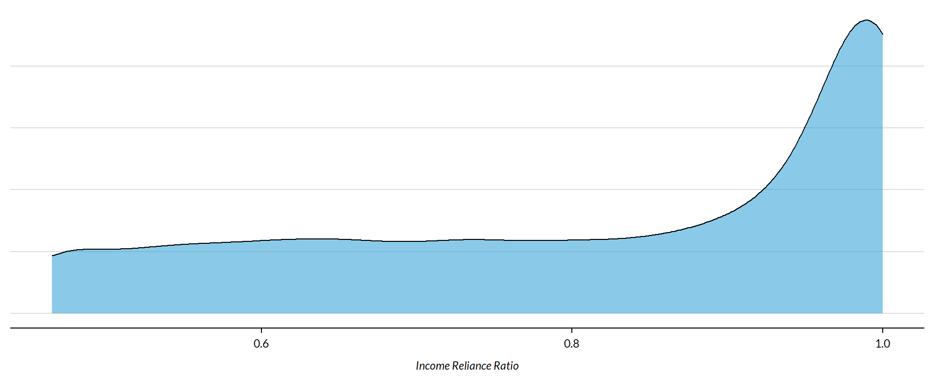

Income Reliance Ratio by NTEE Major Code

core3 <- core2 %>% filter( ! is.na(NTEE1) )
table( core3$NTEE1) %>% sort(decreasing=TRUE) %>% kable()

Var1	Freq
Housing	2837
Community Development	1585
Human Services	1102


t <- table( factor(core3$NTEE1) ) 
df <- data.frame( x=Inf, y=Inf, 
                  N=paste0( "N=", as.character(t) ), 
                  NTEE1=names(t) )

ggplot( core3, aes( x=income_reliance_ratio ) ) + 
  geom_density( alpha = 0.5) + 
  # xlim( -0.1, 1 ) +
  labs( title="Nonprofit Subsectors" ) + 
  xlab( variable.label4 ) + 
  facet_wrap( ~ NTEE1, nrow=1 ) + 
    theme_minimal( base_size = 15 )  + 
    theme( axis.title.y=element_blank(),
           axis.text.y=element_blank(), 
           axis.ticks.y=element_blank(),
           strip.text = element_text( face="bold") ) +  # size=20 
  geom_text( data=df, 
             aes(x, y, label=N ), 
             hjust=2, vjust=3, 
             color="gray60", size=6 )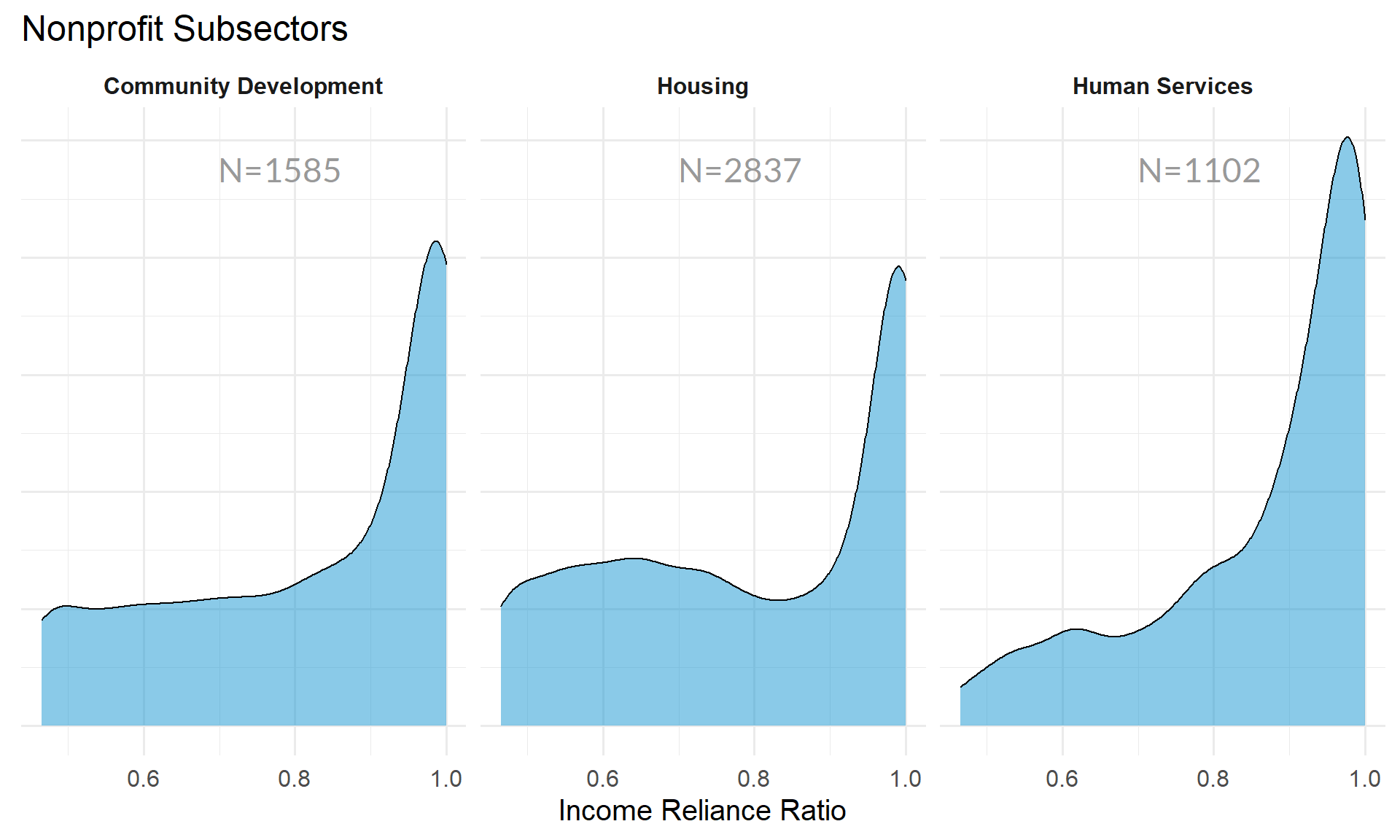

Income Reliance Ratio by Region

table( core2$Region) %>% kable()

Var1	Freq
Midwest	1444
Northeast	1368
South	1610
West	1088

t <- table( factor(core2$Region) ) 
df <- data.frame( x=Inf, y=Inf, 
                  N=paste0( "N=", as.character(t) ), 
                  Region=names(t) )

core2 %>% 
  filter( ! is.na(Region) ) %>% 
  ggplot( aes(income_reliance_ratio) )  + 
    geom_density( alpha = 0.5 ) + 
    xlab( "Census Regions" ) + 
    ylab( variable.label4 ) +
    facet_wrap( ~ Region, nrow=3 ) + 
    theme_minimal( base_size = 22 )  + 
    theme( axis.title.y=element_blank(),
           axis.text.y=element_blank(), 
           axis.ticks.y=element_blank() ) + 
    geom_text( data=df, 
             aes(x, y, label=N ), 
             hjust=2, vjust=3, 
             color="gray60", size=6 )

table( core2$Division ) %>% kable()

Var1	Freq
East North Central	1038
East South Central	289
Middle Atlantic	904
Mountain	303
New England	464
Pacific	785
South Atlantic	900
West North Central	406
West South Central	421

t <- table( factor(core2$Division) ) 
df <- data.frame( x=Inf, y=Inf, 
                  N=paste0( "N=", as.character(t) ), 
                  Division=names(t) )

core2 %>% 
  filter( ! is.na(Division) ) %>% 
  ggplot( aes(income_reliance_ratio) )  + 
    geom_density( alpha = 0.5 ) + 
    xlab( "Census Sub-Regions (10)" ) + 
    ylab( variable.label4 ) +
    facet_wrap( ~ Division, nrow=3 ) + 
    theme_minimal( base_size = 22 )  + 
    theme( axis.title.y=element_blank(),
           axis.text.y=element_blank(), 
           axis.ticks.y=element_blank() ) + 
    geom_text( data=df, 
             aes(x, y, label=N ), 
             hjust=2, vjust=3, 
             color="gray60", size=6 )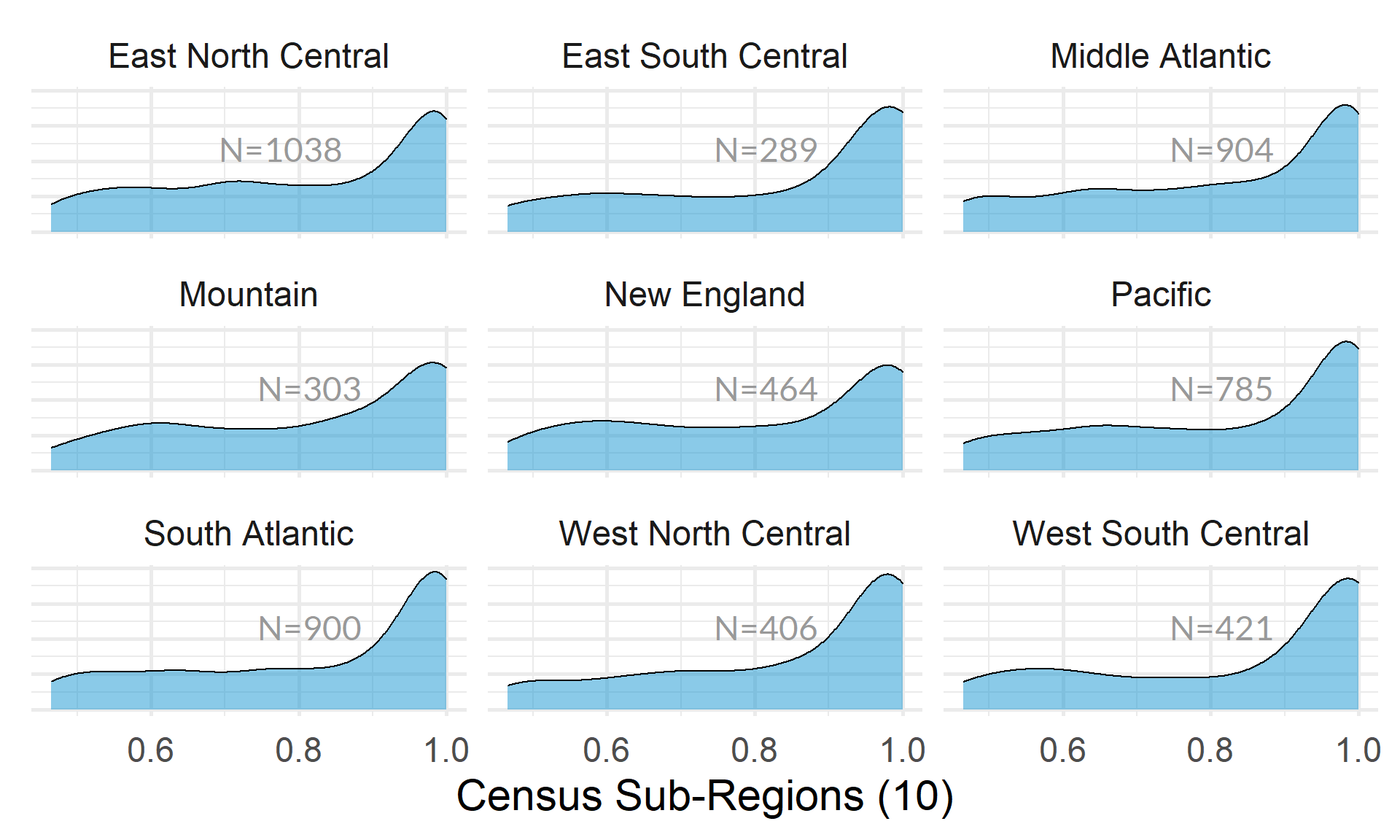

Income Reliance Ratio by Nonprofit Size (Expenses)

ggplot( core2, aes(x = totfuncexpns )) +  
  geom_density( alpha = 0.5 ) + 
  xlim( quantile(core2$totfuncexpns, c(0.02,0.98), na.rm=T ) )

core2$totfuncexpns[ core2$totfuncexpns < 1 ] <- 1
# core2$totfuncexpns[ is.na(core2$totfuncexpns) ] <- 1

if( nrow(core2) > 10000 )
{
  core3 <- sample_n( core2, 10000 )
} else
{
  core3 <- core2
}

jplot( log10(core3$totfuncexpns), core3$income_reliance_ratio, 
       xlab="Nonprofit Size (logged Expenses)", 
       ylab=variable.label4,
       xaxt="n", xlim=c(3,10) )
axis( side=1, 
      at=c(3,4,5,6,7,8,9,10), 
      labels=c("1k","10k","100k","1m","10m","100m","1b","10b") )

core2 %>% 
  filter( ! is.na(exp.q) ) %>% 
  ggplot( aes(income_reliance_ratio) )  + 
    geom_density( alpha = 0.5) + 
    labs( title="Nonprofit Size (logged expenses)" ) + 
    xlab( variable.label4 ) +
    facet_wrap( ~ exp.q, nrow=3 ) + 
    theme_minimal( base_size = 22 )  + 
    theme( axis.title.y=element_blank(),
           axis.text.y=element_blank(), 
           axis.ticks.y=element_blank() )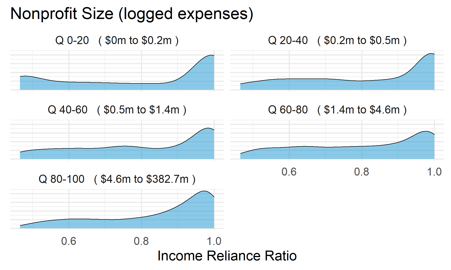

Income Reliance Ratio by Nonprofit Size (Revenue)

ggplot( core2, aes(x = totrevenue )) +  
  geom_density( alpha = 0.5 ) + 
  xlim( quantile(core2$totrevenue, c(0.02,0.98), na.rm=T ) ) + 
  theme( axis.title.y=element_blank(),
           axis.text.y=element_blank(), 
           axis.ticks.y=element_blank() )

core2$totrevenue[ core2$totrevenue < 1 ] <- 1

if( nrow(core2) > 10000 )
{
  core3 <- sample_n( core2, 10000 )
} else
{
  core3 <- core2
}

jplot( log10(core3$totrevenue), core3$income_reliance_ratio, 
       xlab="Nonprofit Size (logged Revenue)", 
       ylab=variable.label4,
       xaxt="n", xlim=c(3,10) )
axis( side=1, 
      at=c(3,4,5,6,7,8,9,10), 
      labels=c("1k","10k","100k","1m","10m","100m","1b","10b") )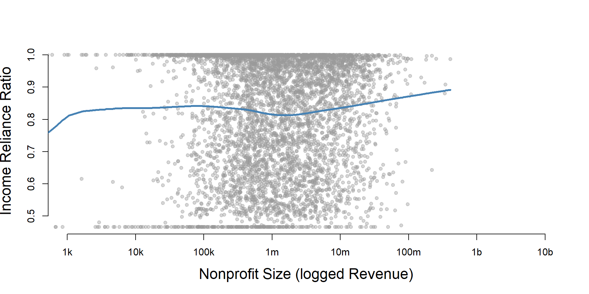

core2 %>% 
  filter( ! is.na(rev.q) ) %>% 
  ggplot( aes(income_reliance_ratio) )  + 
    geom_density( alpha = 0.5 ) + 
    labs( title="Nonprofit Size (logged revenues)" ) + 
    xlab( variable.label4 ) +
    facet_wrap( ~ rev.q, nrow=3 ) + 
    theme_minimal( base_size = 22 )  + 
    theme( axis.title.y=element_blank(),
           axis.text.y=element_blank(), 
           axis.ticks.y=element_blank() )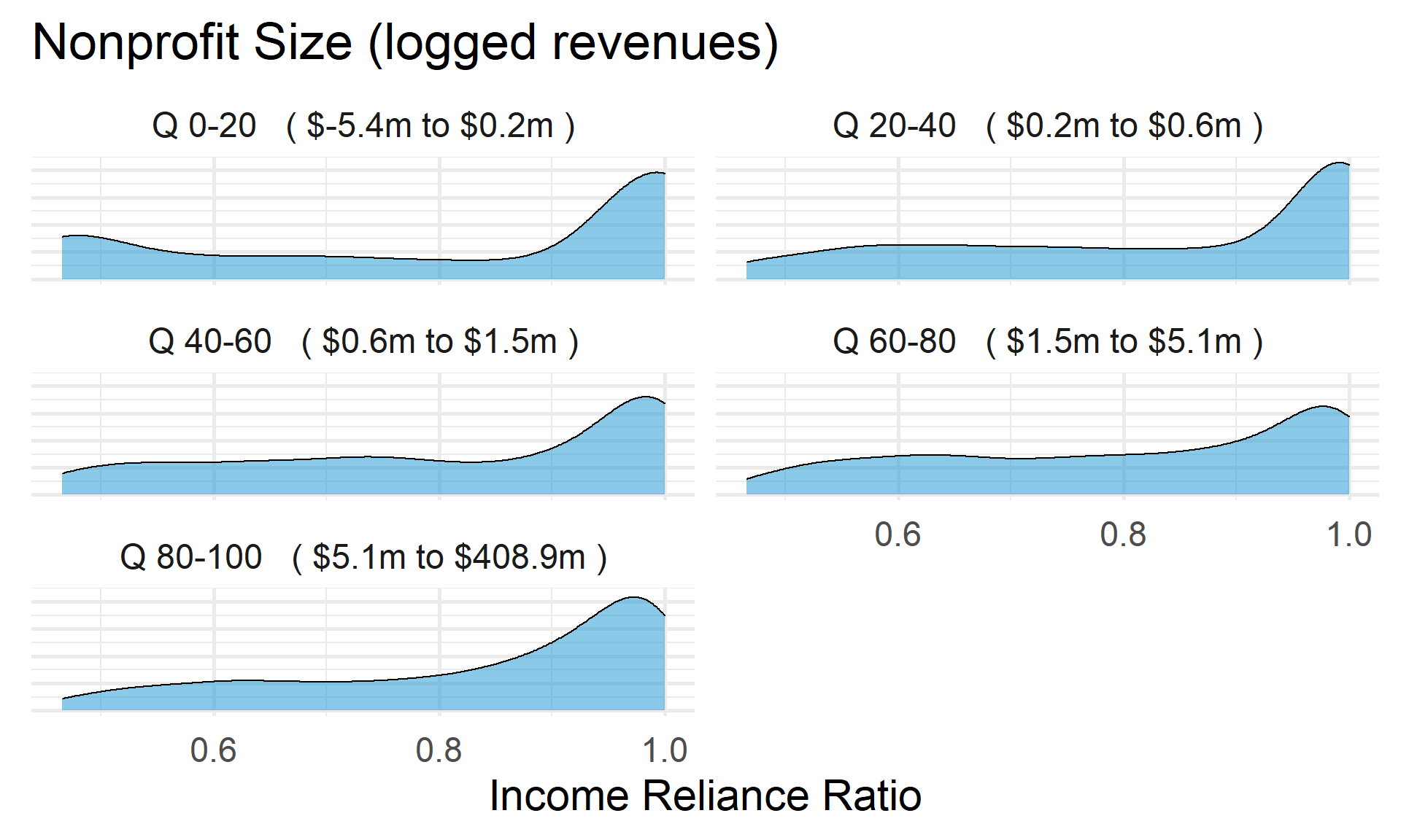

Income Reliance Ratio by Nonprofit Size (Net Assets)

ggplot( core2, aes(x = totnetassetend )) +  
  geom_density( alpha = 0.5) + 
  xlim( quantile(core2$totnetassetend, c(0.02,0.98), na.rm=T ) ) + 
  xlab( "Net Assets" ) +
    theme( axis.title.y=element_blank(),
           axis.text.y=element_blank(), 
           axis.ticks.y=element_blank() )

core2$totnetassetend[ core2$totnetassetend < 1 ] <- NA

if( nrow(core2) > 10000 )
{
  core3 <- sample_n( core2, 10000 )
} else
{
  core3 <- core2
}

jplot( log10(core3$totnetassetend), core3$income_reliance_ratio, 
       xlab="Nonprofit Size (logged Net Assets)", 
       ylab=variable.label4,
       xaxt="n", xlim=c(3,10) )
axis( side=1, 
      at=c(3,4,5,6,7,8,9,10), 
      labels=c("1k","10k","100k","1m","10m","100m","1b","10b") )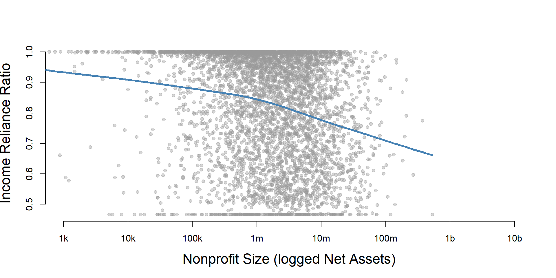

core2$totnetassetend[ core2$totnetassetend < 1 ] <- NA
core2$asset.q <- create_quantiles( var=core2$totnetassetend, n.groups=5 )

core2 %>% 
  filter( ! is.na(asset.q) ) %>% 
  ggplot( aes(income_reliance_ratio) )  + 
    geom_density( alpha = 0.5 ) + 
    labs( title="Nonprofit Size (logged net assets, if assets > 0)" ) + 
    xlab( variable.label4 ) + 
    ylab( "" ) + 
    facet_wrap( ~ asset.q, nrow=3 ) + 
    theme_minimal( base_size = 22 )  + 
    theme( axis.title.y=element_blank(),
           axis.text.y=element_blank(), 
           axis.ticks.y=element_blank() )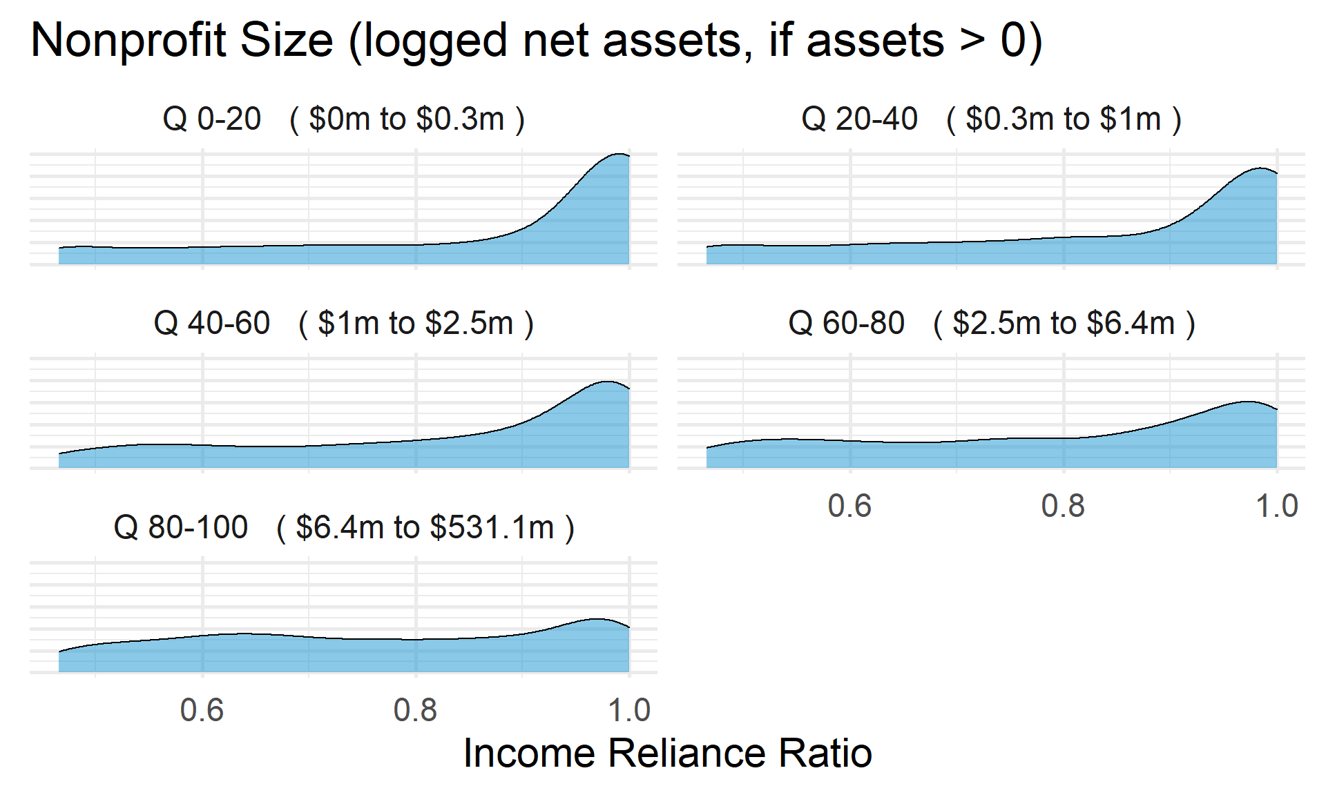

Total Assets for Comparison

core2$totassetsend[ core2$totassetsend < 1 ] <- NA
core2$tot.asset.q <- create_quantiles( var=core2$totassetsend, n.groups=5 )

if( nrow(core2) > 10000 )
{
  core3 <- sample_n( core2, 10000 )
} else
{
  core3 <- core2
}

jplot( log10(core3$totassetsend), core3$income_reliance_ratio, 
       xlab="Nonprofit Size (logged Total Assets)", 
       ylab=variable.label4,
       xaxt="n", xlim=c(3,10) )
axis( side=1, 
      at=c(3,4,5,6,7,8,9,10), 
      labels=c("1k","10k","100k","1m","10m","100m","1b","10b") )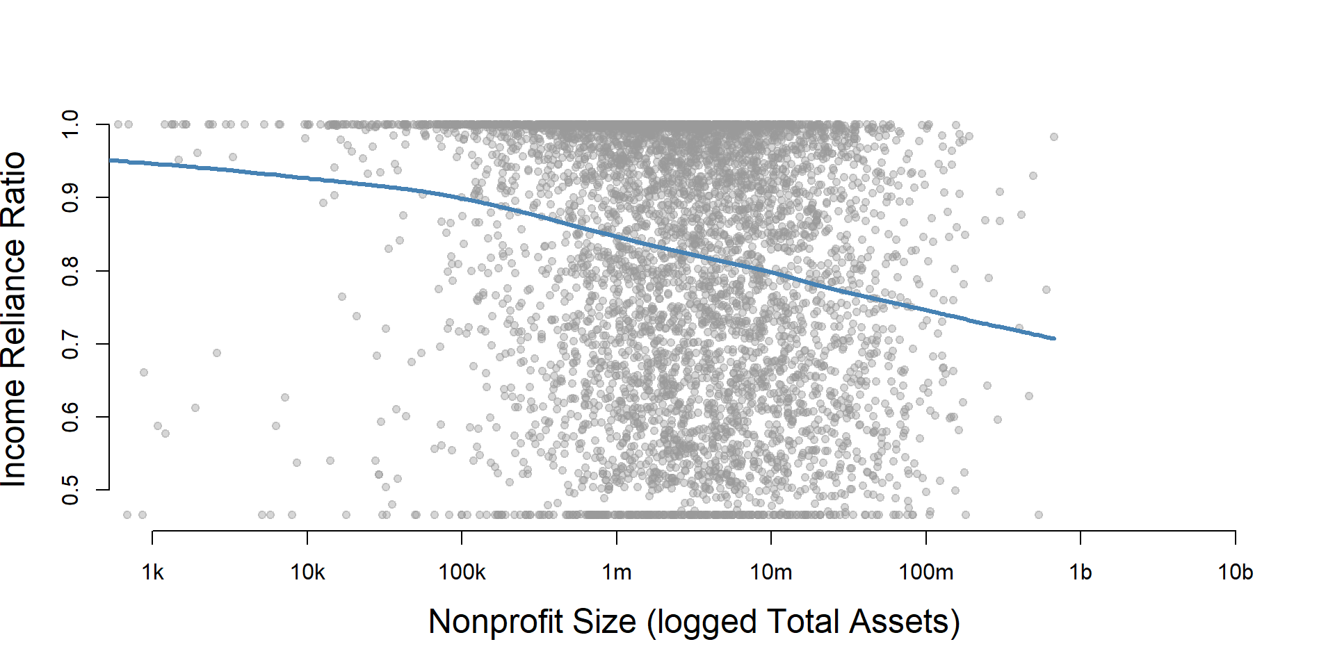

ggplot( core2, aes(x = totassetsend )) +  
  geom_density( alpha = 0.5) + 
  xlim( quantile(core2$totassetsend, c(0.02,0.98), na.rm=T ) ) + 
  xlab( "Net Assets" ) +
    theme( axis.title.y=element_blank(),
           axis.text.y=element_blank(), 
           axis.ticks.y=element_blank() )

core2 %>% 
  filter( ! is.na(tot.asset.q) ) %>% 
  ggplot( aes(income_reliance_ratio) )  + 
    geom_density( alpha = 0.5 ) + 
    xlab( "Nonprofit Size (logged total assets, if assets > 0)" ) + 
    ylab( variable.label4 ) +
    facet_wrap( ~ tot.asset.q, nrow=3 ) + 
    theme_minimal( base_size = 22 )  + 
    theme( axis.title.y=element_blank(),
           axis.text.y=element_blank(), 
           axis.ticks.y=element_blank() )

Income Reliance Ratio by Nonprofit Age

ggplot( core2, aes(x = AGE )) +  
  geom_density( alpha = 0.5 )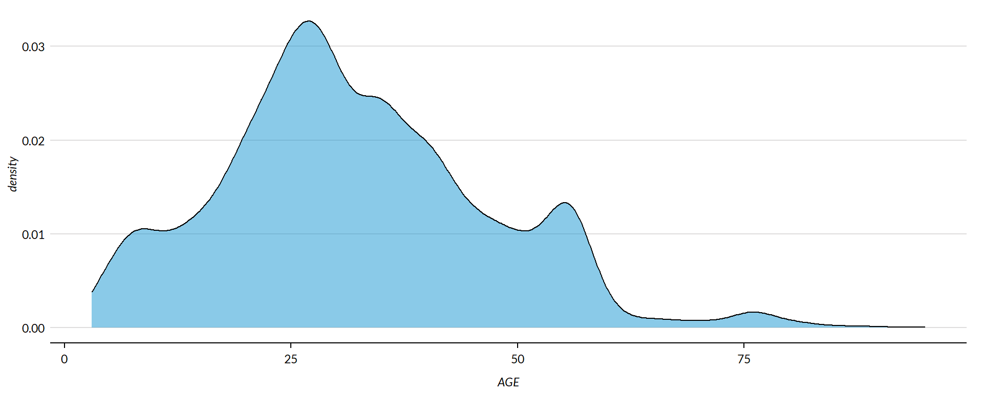

core2$AGE[ core2$AGE < 1 ] <- NA

if( nrow(core2) > 10000 )
{
  core3 <- sample_n( core2, 10000 )
} else
{
  core3 <- core2
}

jplot( core3$AGE, core3$income_reliance_ratio, 
       xlab="Nonprofit Age", 
       ylab=variable.label4 )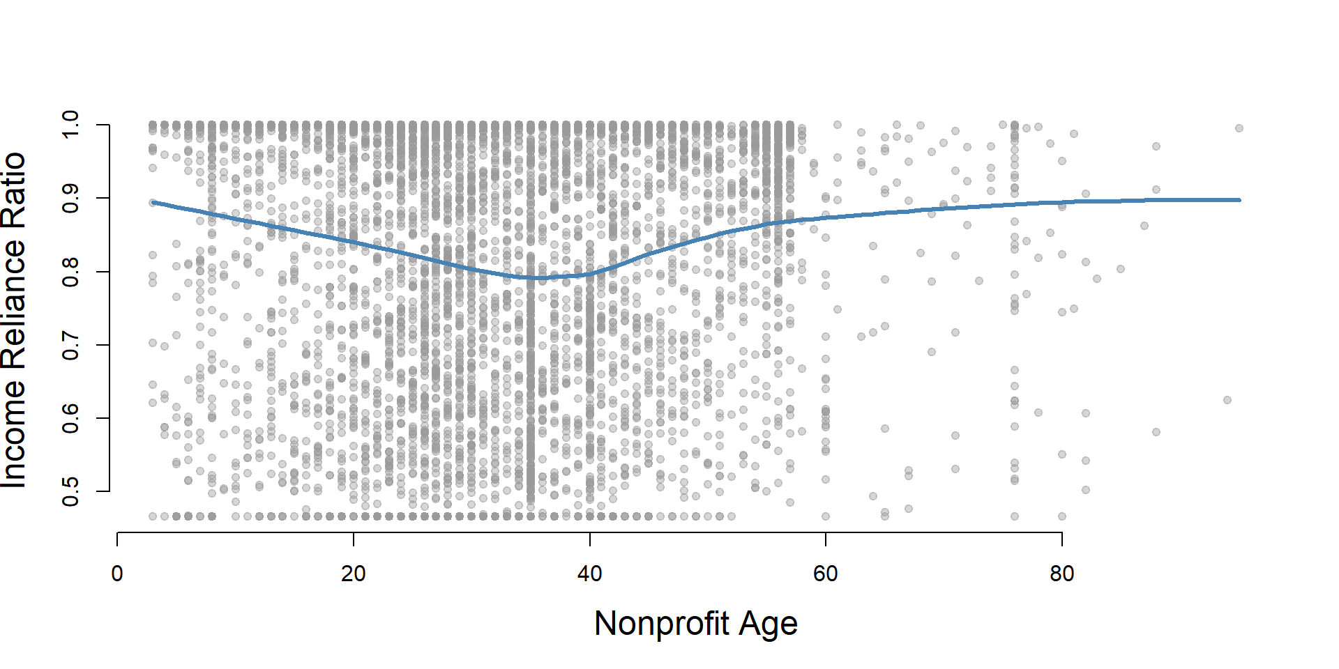

core2 %>% 
  filter( ! is.na(age.q) ) %>% 
  ggplot( aes(income_reliance_ratio) )  + 
    geom_density( alpha = 0.5 ) + 
    labs( title="Nonprofit Age" ) + 
    xlab( variable.label4 ) +
    ylab( "" ) +
    facet_wrap( ~ age.q, nrow=3 ) + 
    theme_minimal( base_size = 22 )  + 
    theme( axis.title.y=element_blank(),
           axis.text.y=element_blank(), 
           axis.ticks.y=element_blank() )

Income Reliance Ratio by Land and Building Value

ggplot( core2, aes(x = lndbldgsequipend )) +  
  geom_density( alpha = 0.5 )

core2$lndbldgsequipend[ core2$lndbldgsequipend < 1 ] <- NA
if( nrow(core2) > 10000 )
{
  core3 <- sample_n( core2, 10000 )
} else
{
  core3 <- core2


jplot( log10(core3$lndbldgsequipend), core3$income_reliance_ratio, 
       xlab="Land and Building Value (logged)", 
       ylab=variable.label4,
       xaxt="n", xlim=c(3,10) )
axis( side=1, 
      at=c(3,4,5,6,7,8,9,10), 
      labels=c("1k","10k","100k","1m","10m","100m","1b","10b") )
}

core2 %>% 
  filter( ! is.na(land.q) ) %>% 
  ggplot( aes(income_reliance_ratio) )  + 
    geom_density( alpha = 0.5 ) + 
    labs( title="Land and Building Value" ) + 
    xlab( variable.label4 ) +
    ylab( "" ) +
    facet_wrap( ~ land.q, nrow=3 ) + 
    theme_minimal( base_size = 22 )  + 
    theme( axis.title.y=element_blank(),
           axis.text.y=element_blank(), 
           axis.ticks.y=element_blank() )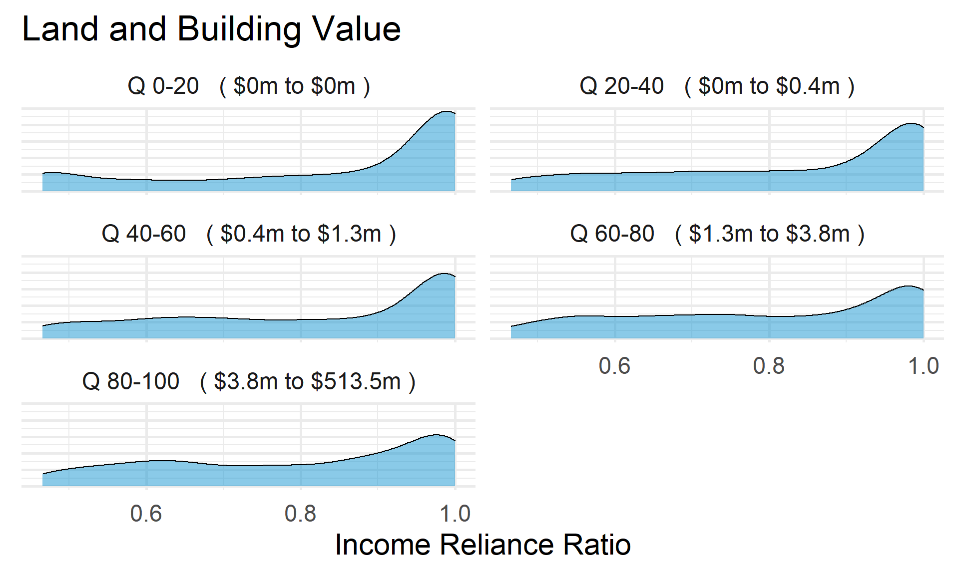

Save Metrics

core.donation_ratio <- select( core, ein, tax_pd, donation_ratio )
saveRDS( core.donation_ratio, "03-data-ratios/m-14-income-reliance-ratios.rds" )
write.csv( core.donation_ratio, "03-data-ratios/m-14-income-reliance-ratios.csv" )

Metric 14-Income Reliance Ratios

April 8, 2022

Metric Construction

Definition & Interpretation

Donation/Grant Dependence Ratio

Investment Income Dependence Ratio

Income Reliance Ratio

Variables

Donation/Grant Dependence Ratio

Earned Income Dependence Ratio

Investment Income Dependence Ratio

Donation/Grant Reliance Ratio Analysis

Standardize Scales

Metric Scope

Descriptive Statistics

Donated Income Dependence Ratio Density

Donated Income Dependence Ratio by NTEE Major Code

Donated Income Dependence Ratio by Region

Donated Income Dependence Ratio by Nonprofit Size (Expenses)

Donated Income Dependence Ratio by Nonprofit Size (Revenue)

Donated Income Dependence Ratio by Nonprofit Size (Net Assets)

Donated Income Dependence Ratio by Nonprofit Age

Donated Income Dependence Ratio by Land and Building Value

Earned Income Reliance Ratio Analysis

Standardize Scales

Metric Scope

Descriptive Statistics

Earned Income Dependence Ratio Density

Earned Income Dependence Ratio by NTEE Major Code

Earned Income Dependence Ratio by Region

Earned Income Dependence Ratio by Nonprofit Size (Expenses)

Earned Income Dependence Ratio by Nonprofit Size (Revenue)

Earned Income Dependence Ratio by Nonprofit Size (Net Assets)

Earned Income Dependence Ratio by Nonprofit Age

Earned Income Dependence Ratio by Land and Building Value

Investment Income Reliance Ratio Analysis

Standardize Scales

Metric Scope

Descriptive Statistics

Investment Income Dependence Ratio Density

Investment Income Dependence Ratio by NTEE Major Code

Investment Income Dependence Ratio by Region

Investment Income Dependence Ratio by Nonprofit Size (Expenses)

Investment Income Dependence Ratio by Nonprofit Size (Revenue)

Investment Income Dependence Ratio by Nonprofit Size (Net Assets)

Investment Income Dependence Ratio by Nonprofit Age

Investment Income Dependence Ratio by Land and Building Value

Income Reliance Ratio Analysis

Standardize Scales

Metric Scope

Descriptive Statistics

Income Reliance Ratio Density

Income Reliance Ratio by NTEE Major Code

Income Reliance Ratio by Region

Income Reliance Ratio by Nonprofit Size (Expenses)

Income Reliance Ratio by Nonprofit Size (Revenue)

Income Reliance Ratio by Nonprofit Size (Net Assets)

Income Reliance Ratio by Nonprofit Age

Income Reliance Ratio by Land and Building Value

Save Metrics