Metric 03- Days of Operating Cash on Hand
April 8, 2022
![]()
Metric Construction
Definition & Interpretation
\[Days \: of \: Operating \: Cash \: on \: Hand = \frac{Operating \: Reserves}{[(Operating \: Expenses - Noncash \: Expenses) / 365]} \]
Days cash on hand is the number of days that an organization can continue to pay its operating expenses, given the amount of cash available.
This metric is good to review at startup of organization, during periods of low revenues, and prior to undertaking new major activity.
The metric is limited though in the following ways. First, it is based on an average daily cash outflow, which is not really the case. Instead, cash tends to be spent in a lumpy manner, such as when rent or payroll are paid. Also, management tends to take drastic action to reduce expenses as cash reserves decline, so that the actual days of operation tend to be longer than indicated by this ratio. Thus, it is better to use a detailed cash flow analysis to determine the precise duration of the available cash, with regular updates.
Variables
Note: This data is available only for organizations that file full 990s. [Organizations with revenues <$200,000 and total assets <$500,000 have the option to not file a full 990 and file an EZ instead.]
Numerator: (Cash + short-term investments + current
receivables)
* On 990: (Part X, line 1B) + (Part X, line 2B) +
(Part X, line 3B) + (Part X, line 4B) - SOI PC EXTRACTS: nonintcashend,
svngstempinvend, pldgegrntrcvblend, accntsrcvblend
* On EZ:Part I,
line 22 [cash and short-term investments only] - SOI PC EXTRACTS: Not
available
Denominator: ((Operating expenses – bad
debts – depreciation) / 365) * On 990: Part IX, line 25A – Part IX, line
22A -SOI PC EXTRACTS: totfuncexpns-deprcatndepletn * On EZ: Part I, line
17 [operating expenses only]
Note: The original ratio yields years of cash on hand. We divide the denominator by 365, or multiply the ratio by 365, to get days of cash on hand. o The 990 doesn’t record bad debts (the amount listed as uncollectible for receivable accounts); it just asks organizations to report grants/pledges/accounts receivable net of bad debts, so this term is missing from the denominator
operating_cash <- ( core$nonintcashend + core$svngstempinvend +
                         core$pldgegrntrcvblend + core$accntsrcvblend)

# can't divide by zero
payables <- ( core$totfuncexpns + core$deprcatndepletn )/365
payables[ payables == 0 ] <- NA

core$daysoperating_coh <-  operating_cash / payables

# summary( core$daysoperating_coh )
Standardize Scales
Check high and low values to see what makes sense.
x.05 <- quantile( core$daysoperating_coh, 0.05, na.rm=T )
x.95 <- quantile( core$daysoperating_coh, 0.95, na.rm=T )

ggplot( core, aes(x = daysoperating_coh ) ) +
  geom_density( alpha = 0.5) +
xlim( x.05, x.95 ) 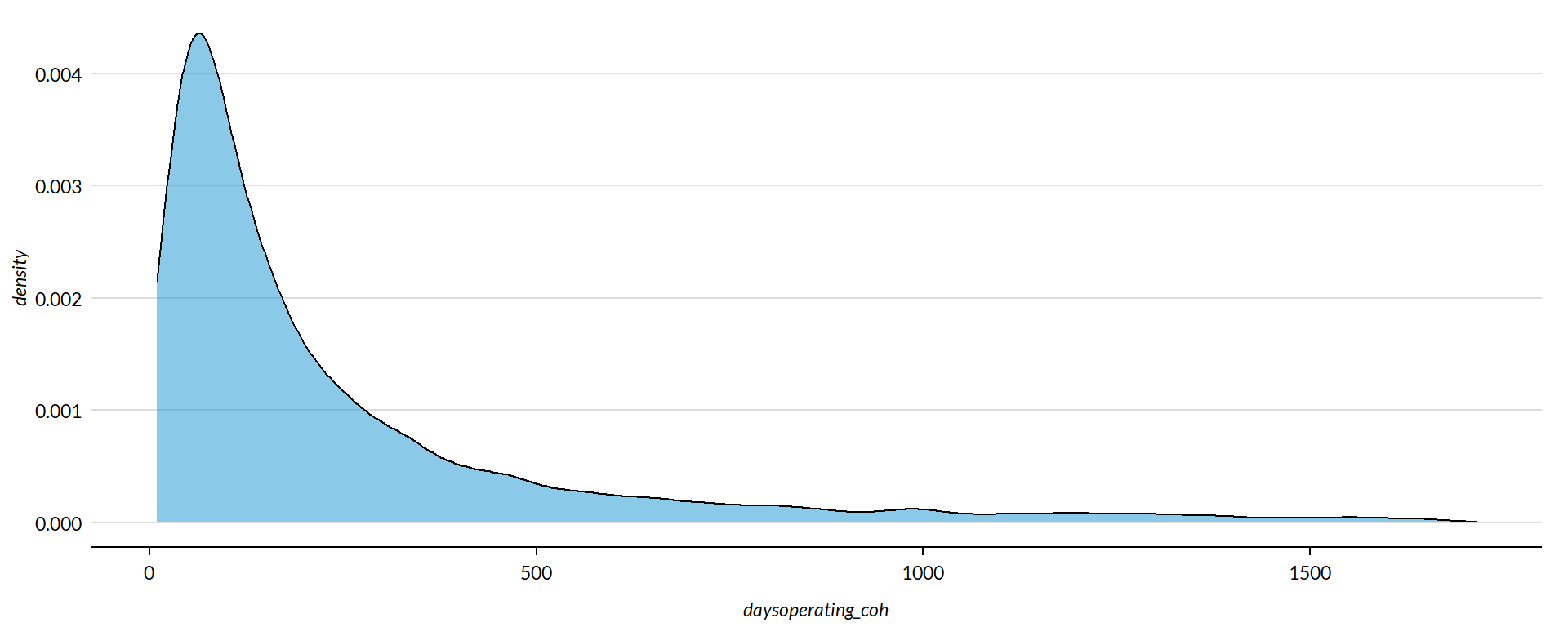
core2 <- core

# proportion of values that are negative
mean( core2$daysoperating_coh < 0, na.rm=T )
## [1] 0.001703255
core2$daysoperating_coh[ core2$daysoperating_coh < 0 ] <- 0

# proption of values above 200%
#mean( core2$daysoperating_coh > 50, na.rm=T )
#core2$daysoperating_coh[ core2$daysoperating_coh > 50 ] <- 50
Metric Scope
Tax data is available for full 990 filers, so this metric does not describe any organizations with Gross receipts < $200,000 and Total assets < $500,000. Some organizations with receipts or assets below those thresholds may have filed a full 990, but these would be exceptions.
Descriptive Statistics
Convert all monetary variables to thousands of dollars.
core2 %>%
  mutate( # daysoperating_coh = daysoperating_coh * 10000,
    totrevenue = totrevenue / 1000,
    totfuncexpns = totfuncexpns / 1000,
    lndbldgsequipend = lndbldgsequipend / 1000,
    totassetsend = totassetsend / 1000,
    totliabend = totliabend / 1000,
    totnetassetend = totnetassetend / 1000 ) %>%
  select( STATE,  NTEE1, NTMAJ12,
          daysoperating_coh,
          AGE,
          totrevenue, totfuncexpns,
          lndbldgsequipend, totassetsend,
          totnetassetend, totliabend ) %>%

  stargazer( type = s.type,
             digits=0,
             summary.stat = c("min","p25","median",
                              "mean","p75","max", "sd"),
             covariate.labels = c("Days of Operating COH", "Age",
                                  "Revenue ($1k)", "Expenses($1k)",
                                  "Buildings ($1k)", "Total Assets ($1k)",
"Net Assets ($1k)", "Liabiliies ($1k)"))| Statistic | Min | Pctl(25) | Median | Mean | Pctl(75) | Max | St. Dev. |
| Days of Operating COH | 0 | 60 | 132 | 4,389 | 327 | 9,561,135 | 160,633 |
| Age | 3 | 22 | 30 | 32 | 41 | 95 | 15 |
| Revenue (1k) | -5,377 | 259 | 909 | 4,522 | 3,672 | 408,932 | 14,286 |
| Expenses(1k) | 0 | 263 | 840 | 4,192 | 3,328 | 382,667 | 13,466 |
| Buildings (1k) | -4 | 79 | 824 | 3,504 | 2,868 | 513,509 | 13,210 |
| Total Assets (1k) | -7,552 | 778 | 2,446 | 9,262 | 7,477 | 672,021 | 27,039 |
| Net Assets (1k) | -178,870 | 156 | 1,094 | 4,553 | 4,079 | 531,068 | 15,470 |
| Liabiliies (1k) | -2,707 | 115 | 816 | 4,709 | 3,133 | 705,623 | 18,722 |
What proportion of orgs have Days of Operating Cash equal to zero (no operating cash)?
prop.zero <- mean( core2$daysoperating_coh == 0, na.rm=T )In the sample, 1 percent of the organizations have zero days of operating cash on hand, meaning they could not survive without receivables and program service revenue. These organizations are dropped from subsequent graphs to keep the visualizations clean. The interpretation of the graphics should be the distributions of Days of Operating Cash on Hand for organizations that have some cash on hand.
###
### ADD QUANTILES
###
###   function create_quantiles() defined in r-functions.R

core2$exp.q   <- create_quantiles( var=core2$totfuncexpns,   n.groups=5 )
core2$rev.q   <- create_quantiles( var=core2$totrevenue,     n.groups=5 )
core2$asset.q <- create_quantiles( var=core2$totnetassetend, n.groups=5 )
core2$age.q   <- create_quantiles( var=core2$AGE,            n.groups=5 )
core2$land.q  <- create_quantiles( var=core2$lndbldgsequipend,    n.groups=5 )
Days of Operating Cash on Hand Density
min.x <- min( core2$daysoperating_coh, na.rm=T )
max.x <- max( core2$daysoperating_coh, na.rm=T )

ggplot( core2, aes(x = daysoperating_coh )) +
  geom_density( alpha = 0.5 ) +
  xlim( min.x, max.x  ) +
  xlab( variable.label ) +
  theme( axis.title.y=element_blank(),
         axis.text.y=element_blank(),
         axis.ticks.y=element_blank() )
Days of Operating Cash on Hand by NTEE Major Code
core3 <- core2 %>% filter( ! is.na(NTEE1) )
table( core3$NTEE1) %>% sort(decreasing=TRUE) %>% kable()| Var1 | Freq |
|---|---|
| Housing | 2837 |
| Community Development | 1585 |
| Human Services | 1102 |
t <- table( factor(core3$NTEE1) )
df <- data.frame( x=Inf, y=Inf,
                  N=paste0( "N=", as.character(t) ),
                  NTEE1=names(t) )

ggplot( core3, aes( x=daysoperating_coh ) ) +
  geom_density( alpha = 0.5) +
  # xlim( -0.1, 1 ) +
  labs( title="Nonprofit Subsectors" ) +
  xlab( variable.label ) +
  facet_wrap( ~ NTEE1, nrow=1 ) +
    theme_minimal( base_size = 15 )  +
    theme( axis.title.y=element_blank(),
           axis.text.y=element_blank(),
           axis.ticks.y=element_blank(),
           strip.text = element_text( face="bold") ) +  # size=20
  geom_text( data=df,
             aes(x, y, label=N ),
             hjust=2, vjust=3,
             color="gray60", size=6 )
Days of Operating Cash on Hand by Region
table( core2$Region) %>% kable()| Var1 | Freq |
|---|---|
| Midwest | 1444 |
| Northeast | 1368 |
| South | 1610 |
| West | 1088 |
t <- table( factor(core2$Region) )
df <- data.frame( x=Inf, y=Inf,
                  N=paste0( "N=", as.character(t) ),
                  Region=names(t) )

core2 %>%
  filter( ! is.na(Region) ) %>%
  ggplot( aes(daysoperating_coh) )  +
    geom_density( alpha = 0.5 ) +
    xlab( "Census Regions" ) +
    ylab( variable.label ) +
    facet_wrap( ~ Region, nrow=3 ) +
    theme_minimal( base_size = 22 )  +
    theme( axis.title.y=element_blank(),
           axis.text.y=element_blank(),
           axis.ticks.y=element_blank() ) +
    geom_text( data=df,
             aes(x, y, label=N ),
             hjust=2, vjust=3,
             color="gray60", size=6 )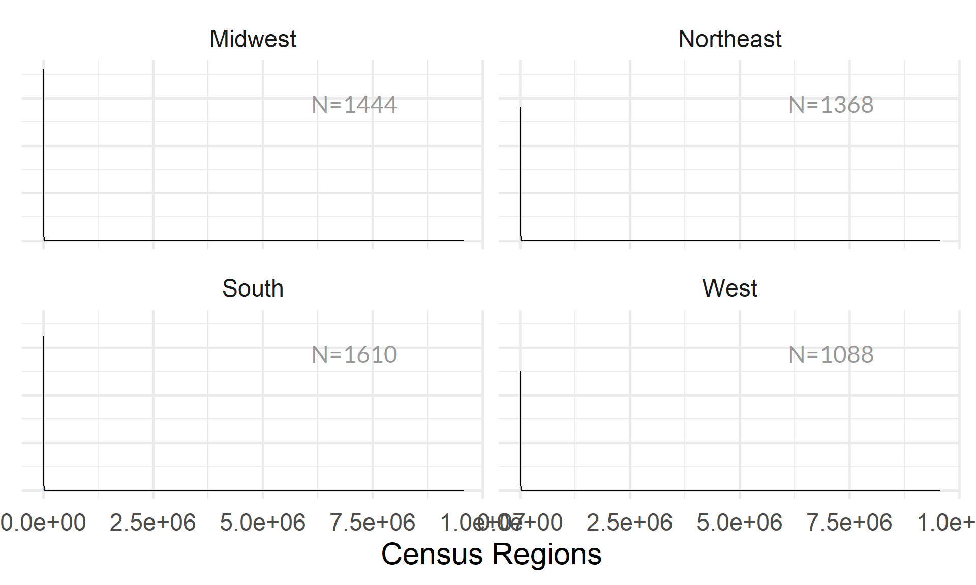
table( core2$Division ) %>% kable()| Var1 | Freq |
|---|---|
| East North Central | 1038 |
| East South Central | 289 |
| Middle Atlantic | 904 |
| Mountain | 303 |
| New England | 464 |
| Pacific | 785 |
| South Atlantic | 900 |
| West North Central | 406 |
| West South Central | 421 |
t <- table( factor(core2$Division) )
df <- data.frame( x=Inf, y=Inf,
                  N=paste0( "N=", as.character(t) ),
                  Division=names(t) )

core2 %>%
  filter( ! is.na(Division) ) %>%
  ggplot( aes(daysoperating_coh) )  +
    geom_density( alpha = 0.5 ) +
    xlab( "Census Sub-Regions (10)" ) +
    ylab( variable.label ) +
    facet_wrap( ~ Division, nrow=3 ) +
    theme_minimal( base_size = 22 )  +
    theme( axis.title.y=element_blank(),
           axis.text.y=element_blank(),
           axis.ticks.y=element_blank() ) +
    geom_text( data=df,
             aes(x, y, label=N ),
             hjust=2, vjust=3,
color="gray60", size=6 ) 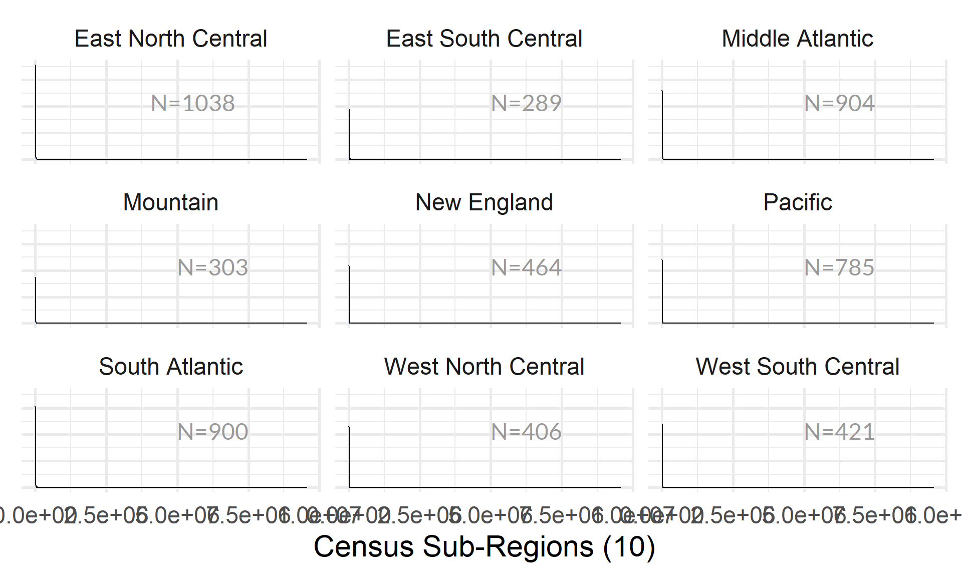
Days of Operating Cash on Hand by Nonprofit Size (Expenses)
ggplot( core2, aes(x = totfuncexpns )) +
  geom_density( alpha = 0.5 ) +
  xlim( quantile(core2$totfuncexpns, c(0.02,0.98), na.rm=T ) )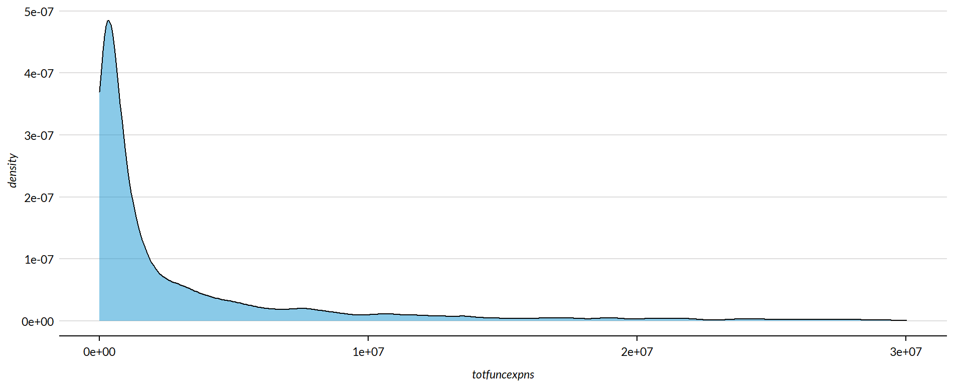
core2$totfuncexpns[ core2$totfuncexpns < 1 ] <- 1
# core2$totfuncexpns[ is.na(core2$totfuncexpns) ] <- 1

if( nrow(core2) > 10000 )
{
  core3 <- sample_n( core2, 10000 )
} else
{
  core3 <- core2
}

jplot( log10(core3$totfuncexpns), core3$daysoperating_coh,
       xlab="Nonprofit Size (logged Expenses)",
       ylab=variable.label,
       xaxt="n", xlim=c(3,10) )
axis( side=1,
      at=c(3,4,5,6,7,8,9,10),
      labels=c("1k","10k","100k","1m","10m","100m","1b","10b") )
core2 %>%
  filter( ! is.na(exp.q) ) %>%
  ggplot( aes(daysoperating_coh) )  +
    geom_density( alpha = 0.5) +
    labs( title="Nonprofit Size (logged expenses)" ) +
    xlab( variable.label ) +
    facet_wrap( ~ exp.q, nrow=3 ) +
    theme_minimal( base_size = 22 )  +
    theme( axis.title.y=element_blank(),
           axis.text.y=element_blank(),
           axis.ticks.y=element_blank() )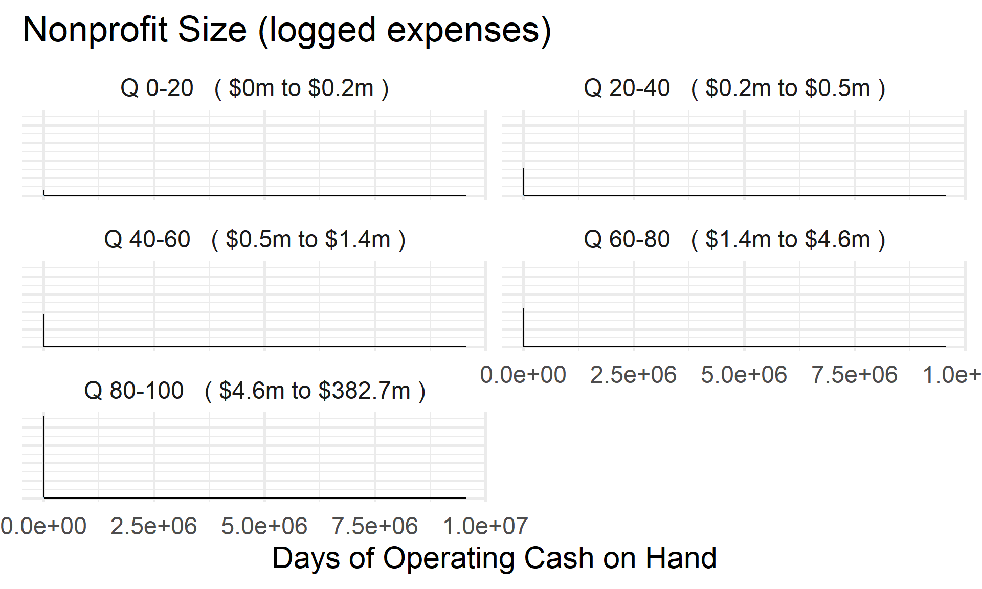
Days of Operating Cash on Hand by Nonprofit Size (Revenue)
ggplot( core2, aes(x = totrevenue )) +
  geom_density( alpha = 0.5 ) +
  xlim( quantile(core2$totrevenue, c(0.02,0.98), na.rm=T ) ) +
  theme( axis.title.y=element_blank(),
           axis.text.y=element_blank(),
           axis.ticks.y=element_blank() )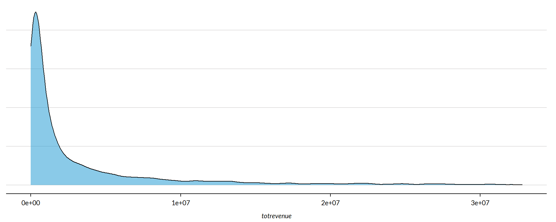
core2$totrevenue[ core2$totrevenue < 1 ] <- 1

if( nrow(core2) > 10000 )
{
  core3 <- sample_n( core2, 10000 )
} else
{
  core3 <- core2
}

jplot( log10(core3$totrevenue), core3$daysoperating_coh,
       xlab="Nonprofit Size (logged Revenue)",
       ylab=variable.label,
       xaxt="n", xlim=c(3,10) )
axis( side=1,
      at=c(3,4,5,6,7,8,9,10),
      labels=c("1k","10k","100k","1m","10m","100m","1b","10b") )
core2 %>%
  filter( ! is.na(rev.q) ) %>%
  ggplot( aes(daysoperating_coh) )  +
    geom_density( alpha = 0.5 ) +
    labs( title="Nonprofit Size (logged revenues)" ) +
    xlab( variable.label ) +
    facet_wrap( ~ rev.q, nrow=3 ) +
    theme_minimal( base_size = 22 )  +
    theme( axis.title.y=element_blank(),
           axis.text.y=element_blank(),
           axis.ticks.y=element_blank() )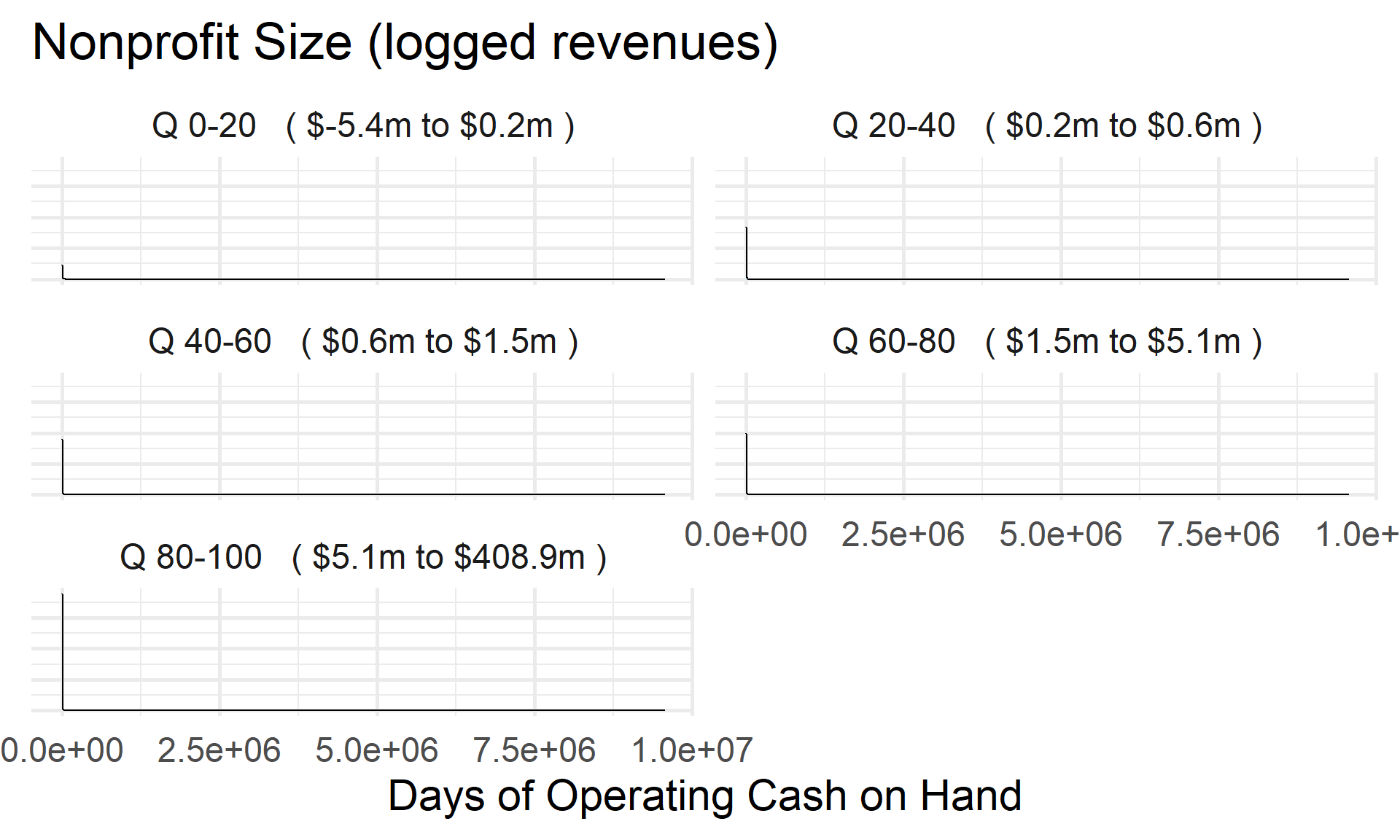
Days of Operating Cash on Hand by Nonprofit Size (Net Assets)
ggplot( core2, aes(x = totnetassetend )) +
  geom_density( alpha = 0.5) +
  xlim( quantile(core2$totnetassetend, c(0.02,0.98), na.rm=T ) ) +
  xlab( "Net Assets" ) +
    theme( axis.title.y=element_blank(),
           axis.text.y=element_blank(),
           axis.ticks.y=element_blank() )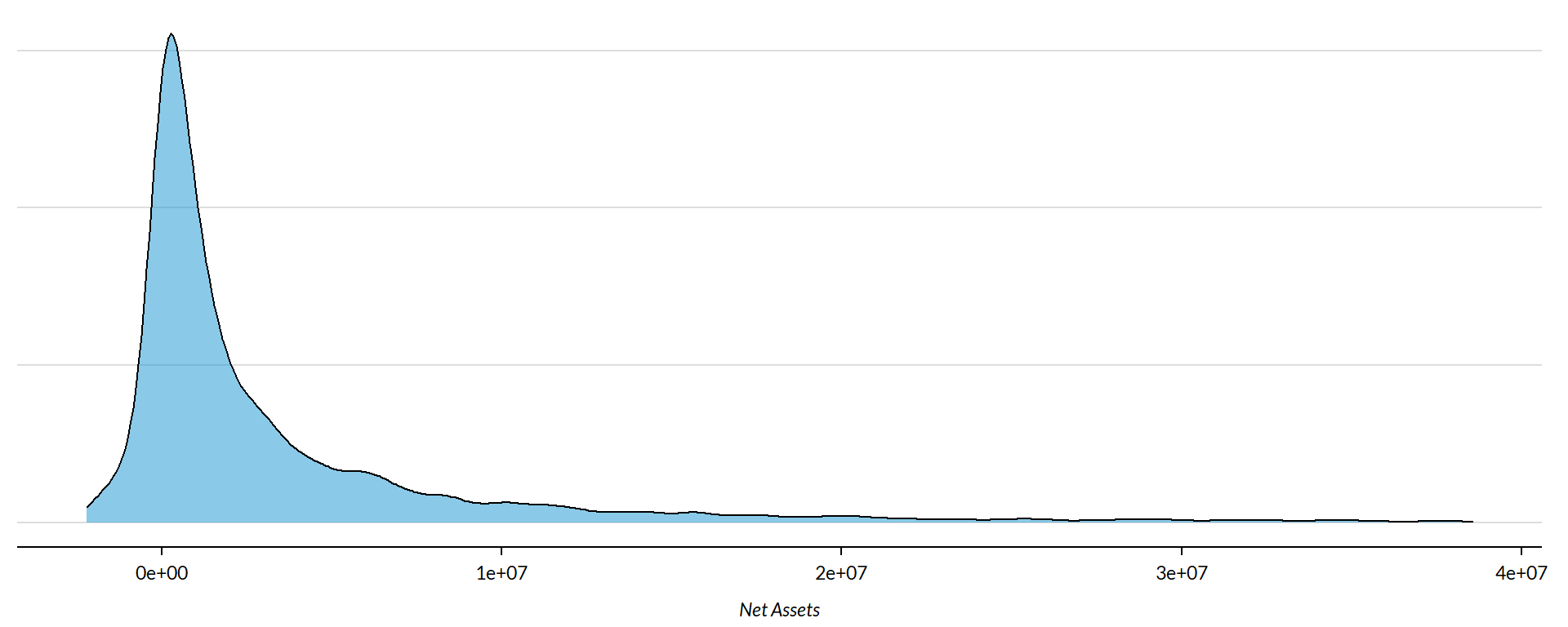
core2$totnetassetend[ core2$totnetassetend < 1 ] <- NA

if( nrow(core2) > 10000 )
{
  core3 <- sample_n( core2, 10000 )
} else
{
  core3 <- core2
}

jplot( log10(core3$totnetassetend), core3$daysoperating_coh,
       xlab="Nonprofit Size (logged Net Assets)",
       ylab=variable.label,
       xaxt="n", xlim=c(3,10) )
axis( side=1,
      at=c(3,4,5,6,7,8,9,10),
      labels=c("1k","10k","100k","1m","10m","100m","1b","10b") )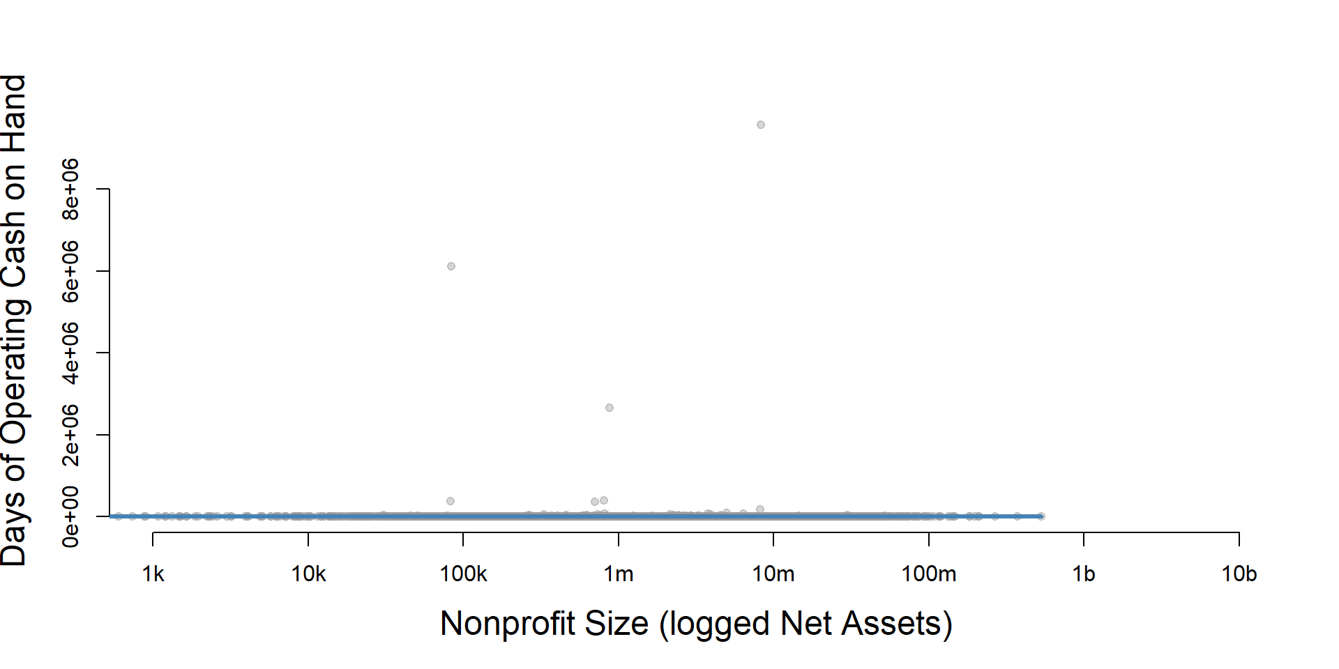
core2$totnetassetend[ core2$totnetassetend < 1 ] <- NA
core2$asset.q <- create_quantiles( var=core2$totnetassetend, n.groups=5 )

core2 %>%
  filter( ! is.na(asset.q) ) %>%
  ggplot( aes(daysoperating_coh) )  +
    geom_density( alpha = 0.5 ) +
    labs( title="Nonprofit Size (logged net assets, if assets > 0)" ) +
    xlab( variable.label ) +
    ylab( "" ) +
    facet_wrap( ~ asset.q, nrow=3 ) +
    theme_minimal( base_size = 22 )  +
    theme( axis.title.y=element_blank(),
           axis.text.y=element_blank(),
           axis.ticks.y=element_blank() )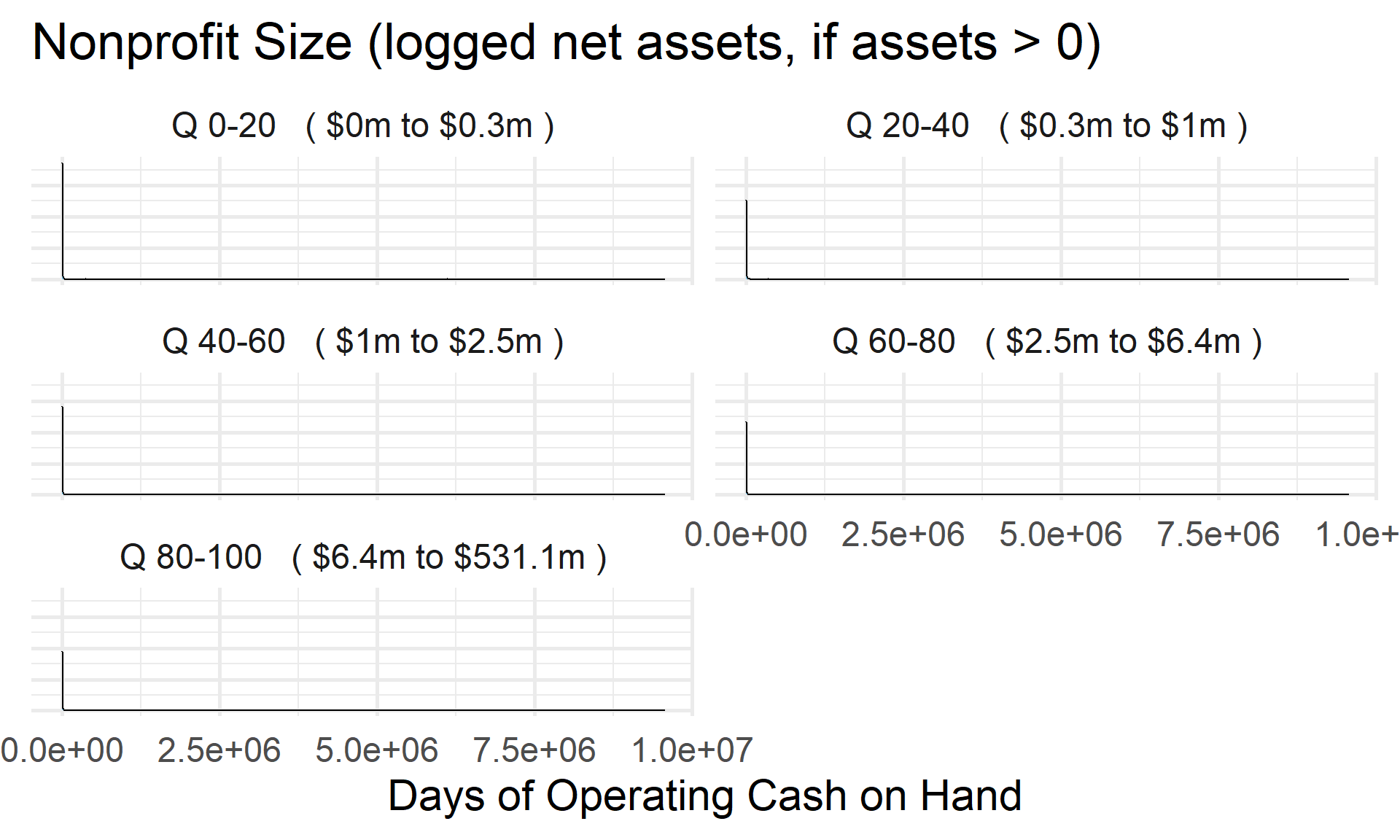
Total Assets for Comparison
core2$totassetsend[ core2$totassetsend < 1 ] <- NA
core2$tot.asset.q <- create_quantiles( var=core2$totassetsend, n.groups=5 )

if( nrow(core2) > 10000 )
{
  core3 <- sample_n( core2, 10000 )
} else
{
  core3 <- core2
}

jplot( log10(core3$totassetsend), core3$daysoperating_coh,
       xlab="Nonprofit Size (logged Total Assets)",
       ylab=variable.label,
       xaxt="n", xlim=c(3,10) )
axis( side=1,
      at=c(3,4,5,6,7,8,9,10),
      labels=c("1k","10k","100k","1m","10m","100m","1b","10b") )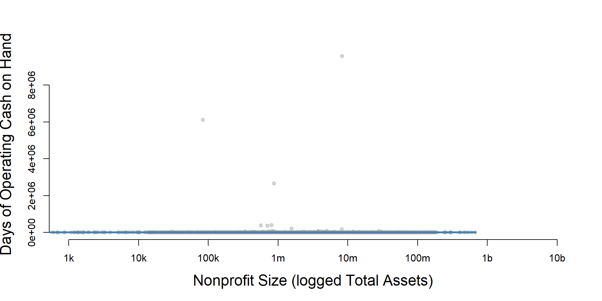
ggplot( core2, aes(x = totassetsend )) +
  geom_density( alpha = 0.5) +
  xlim( quantile(core2$totassetsend, c(0.02,0.98), na.rm=T ) ) +
  xlab( "Net Assets" ) +
    theme( axis.title.y=element_blank(),
           axis.text.y=element_blank(),
           axis.ticks.y=element_blank() )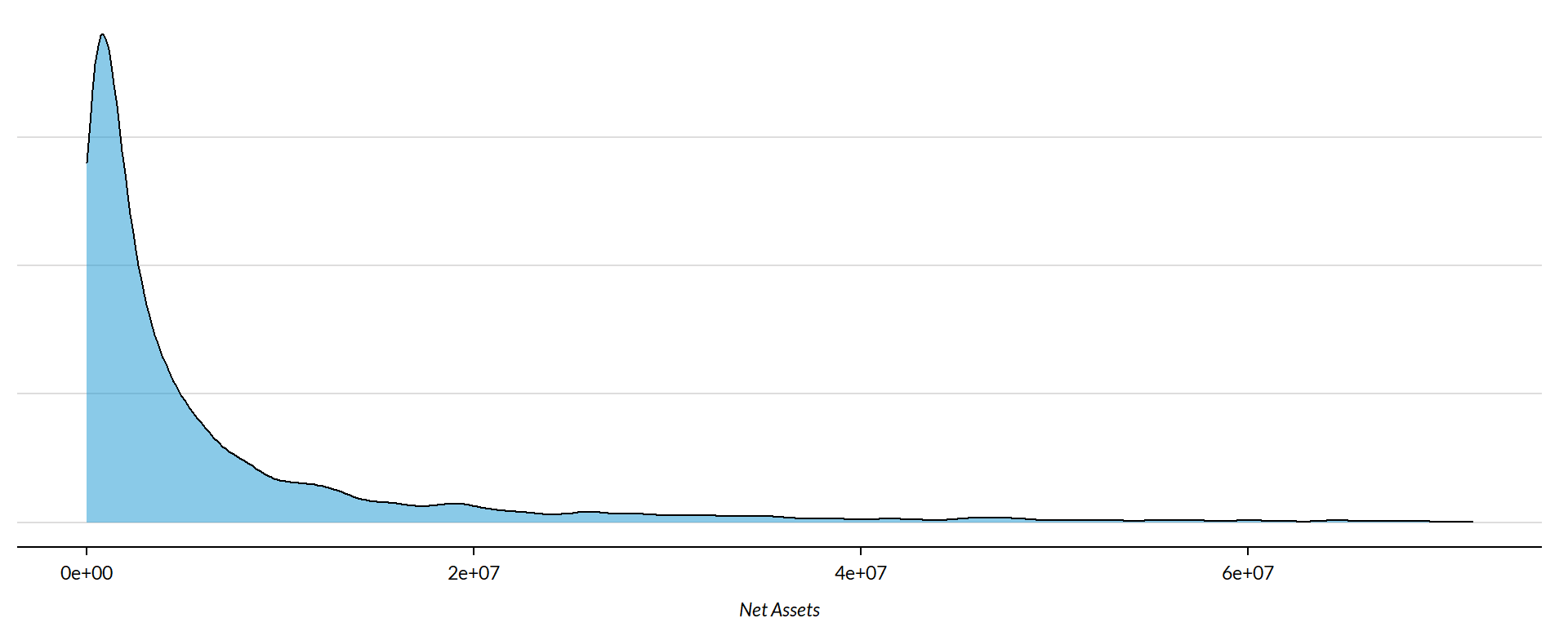
core2 %>%
  filter( ! is.na(tot.asset.q) ) %>%
  ggplot( aes(daysoperating_coh) )  +
    geom_density( alpha = 0.5 ) +
    xlab( "Nonprofit Size (logged total assets, if assets > 0)" ) +
    ylab( variable.label ) +
    facet_wrap( ~ tot.asset.q, nrow=3 ) +
    theme_minimal( base_size = 22 )  +
    theme( axis.title.y=element_blank(),
           axis.text.y=element_blank(),
           axis.ticks.y=element_blank() )
Days of Operating Cash on Hand by Nonprofit Age
ggplot( core2, aes(x = AGE )) +
geom_density( alpha = 0.5 ) 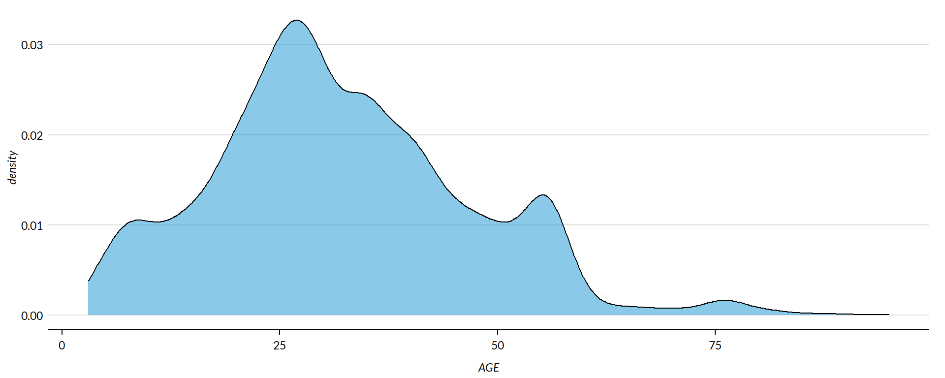
core2$AGE[ core2$AGE < 1 ] <- NA

if( nrow(core2) > 10000 )
{
  core3 <- sample_n( core2, 10000 )
} else
{
  core3 <- core2
}

jplot( core3$AGE, core3$daysoperating_coh,
       xlab="Nonprofit Age",
ylab=variable.label ) 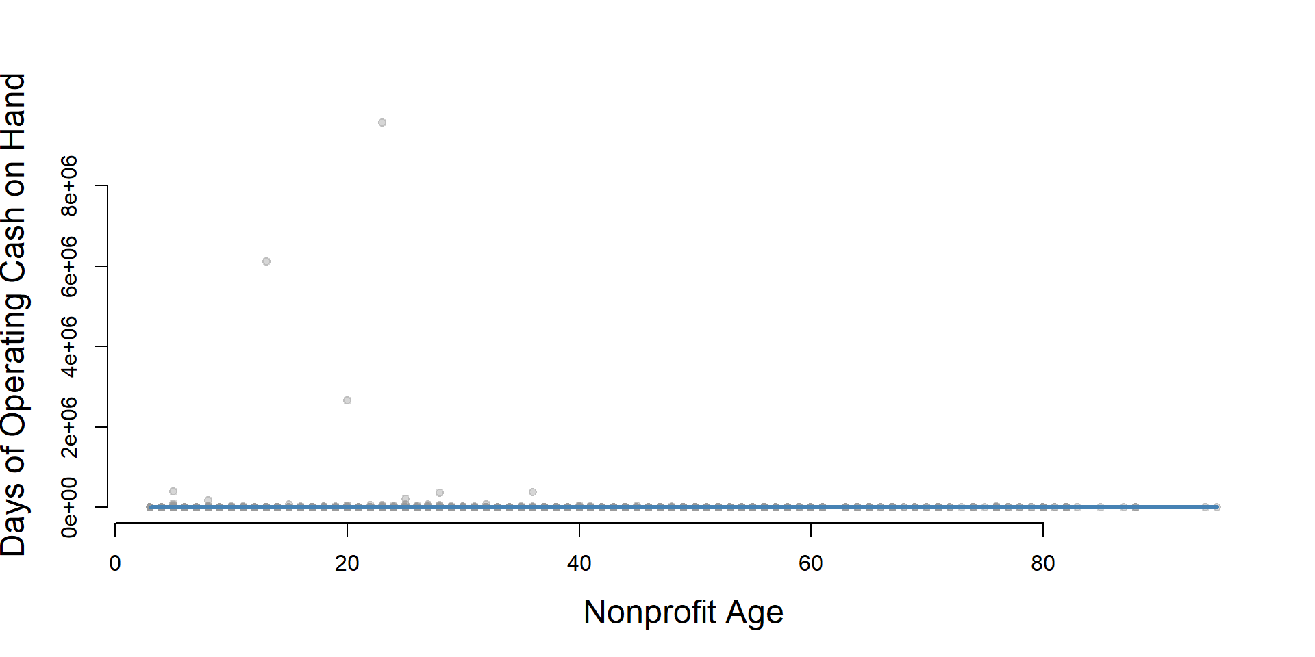
core2 %>%
  filter( ! is.na(age.q) ) %>%
  ggplot( aes(daysoperating_coh) )  +
    geom_density( alpha = 0.5 ) +
    labs( title="Nonprofit Age" ) +
    xlab( variable.label ) +
    ylab( "" ) +
    facet_wrap( ~ age.q, nrow=3 ) +
    theme_minimal( base_size = 22 )  +
    theme( axis.title.y=element_blank(),
           axis.text.y=element_blank(),
           axis.ticks.y=element_blank() )
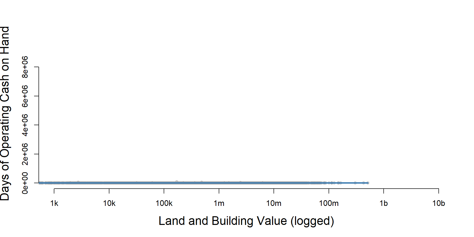
Days of Operating Cash on Hand by Land and Building Value
ggplot( core2, aes(x = lndbldgsequipend )) +
geom_density( alpha = 0.5 ) 
core2$lndbldgsequipend[ core2$lndbldgsequipend < 1 ] <- NA
if( nrow(core2) > 10000 )
{
  core3 <- sample_n( core2, 10000 )
} else
{
  core3 <- core2


jplot( log10(core3$lndbldgsequipend), core3$daysoperating_coh,
       xlab="Land and Building Value (logged)",
       ylab=variable.label,
       xaxt="n", xlim=c(3,10) )
axis( side=1,
      at=c(3,4,5,6,7,8,9,10),
      labels=c("1k","10k","100k","1m","10m","100m","1b","10b") )
}
core2 %>%
  filter( ! is.na(land.q) ) %>%
  ggplot( aes(daysoperating_coh) )  +
    geom_density( alpha = 0.5 ) +
    labs( title="Land and Building Value" ) +
    xlab( variable.label ) +
    ylab( "" ) +
    facet_wrap( ~ land.q, nrow=3 ) +
    theme_minimal( base_size = 22 )  +
    theme( axis.title.y=element_blank(),
           axis.text.y=element_blank(),
           axis.ticks.y=element_blank() )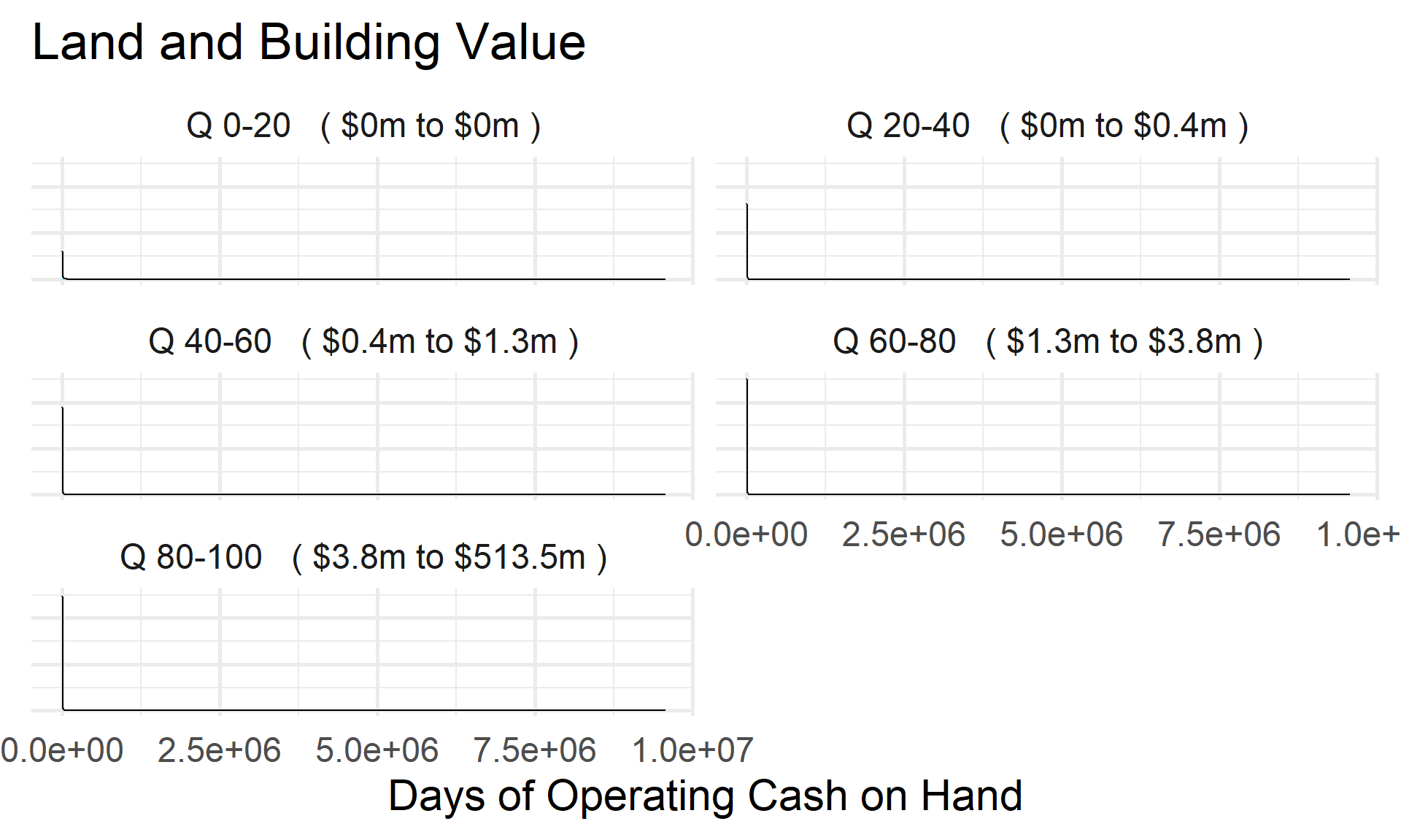
Save Metrics
core.daysoperating_coh <- select( core, ein, tax_pd, daysoperating_coh )
saveRDS( core.daysoperating_coh, "03-data-ratios/m-03-days-operating-cash.rds" )
write.csv( core.daysoperating_coh, "03-data-ratios/m-03-days-operating-cash.csv" )