Metric 04 - Debt to Equity Ratio
April 8, 2022
![]()
Metric Construction
Definition & Interpretation
\[Debt \: to \: Equity \: Ratio = \frac{Total \: Debt}{Unrestricted \: Net \: Assets} \]
Debt to Equity Ratio is a a leverage ratio that defines the total amount of debt relative to the unrestricted assets owned by an organization.
This metric shows the big picture view of how much an organization owes relative to what it owns. Higher values mean it is more highly leveraged, meaning it has low capacity for future borrowing. As an example: if an organization has a total-debt-to-net-assets ratio of 0.4, 40% of its assets are financed by creditors, and 60% are its own unrestricted, available equity. As this percentage creeps above the 50% mark, it can call into question the organization’s ability to manage debt, which could jeopardize the delivery of programs and services. However, for developers, extremely low values may mean the organization is not capitalizing enough on its equity to expand.
This value can be negative if an organization has either overpaid on its debts or if it has negative unrestricted net assets.
One limitation of this metric is that it does not provide any indication of asset quality or liquidity since it lumps tangible and intangible assets together.
Variables
Note: This data is available only for organizations that file full 990s. [Organizations with revenues <$200,000 and total assets <$500,000 have the option to not file a full 990 and file an EZ instead.]
Numerator: Total debt, EOY
* On 990: Part X,
line 17B - SOI PC EXTRACTS: accntspayableend * On EZ: Not Available
Denominator: Unrestricted Net Assets, EOY * On 990:
Part X, line 27B -SOI PC EXTRACTS: unrstrctnetasstsend * On EZ: Not
available
Note: This ratio can be interchanged with total liabilities over total net assets (which should be comparable for EZ filers and full 990 filers), but for Community Development Corporations, the more important metric is unrestricted net assets, which isn’t available for EZ filers.
total_debt <- ( core$accntspayableend )

# can't divide by zero
unrs_net_assets <- (core$unrstrctnetasstsend )
unrs_net_assets[ unrs_net_assets == 0 ] <- NA


core$der <- ( total_debt / unrs_net_assets )
# summary( core$der )
Standardize Scales
Check high and low values to see what makes sense.
x.05 <- quantile( core$der, 0.05, na.rm=T )
x.95 <- quantile( core$der, 0.95, na.rm=T )

ggplot( core, aes(x = der ) ) +
  geom_density( alpha = 0.5) +
xlim( x.05, x.95 ) 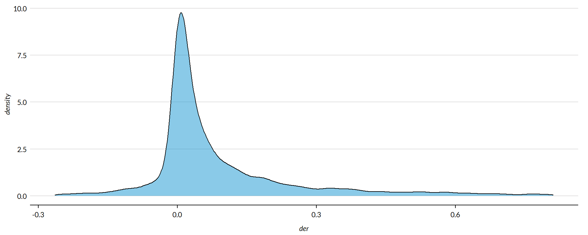
Winsorization: All extreme values have been capped by replacing any values below the 5% distribution and above the 95% distribution with the 5% and 95% values. Consequently the end tails to all density charts may be slightly higher than normal but the tails will not show outliers.
x.05 <- quantile( core$der, 0.05, na.rm=T )
x.95 <- quantile( core$der, 0.95, na.rm=T )

core2 <- core

# proportion of values that are negative
# mean( core2$der < 0, na.rm=T )

# proption of values above 1%
# mean( core2$der > 5, na.rm=T )

# WINSORIZATION AT 5th and 95th PERCENTILES

core2$der[ core2$der < x.05 ] <- x.05
core2$der[ core2$der > x.95 ] <- x.95
Metric Scope
Tax data is available for full 990 filers, so this metric does not describe any organizations with Gross receipts < $200,000 and Total assets < $500,000. Some organizations with receipts or assets below those thresholds may have filed a full 990, but these would be exceptions.
Descriptive Statistics
Convert all monetary variables to thousands of dollars.
core2 %>%
  mutate( der = der * 10000,
    totrevenue = totrevenue / 1000,
    totfuncexpns = totfuncexpns / 1000,
    lndbldgsequipend = lndbldgsequipend / 1000,
    totassetsend = totassetsend / 1000,
    totliabend = totliabend / 1000,
    totnetassetend = totnetassetend / 1000 ) %>%
  select( STATE,  NTEE1, NTMAJ12,
          der,
          AGE,
          totrevenue, totfuncexpns,
          lndbldgsequipend, totassetsend,
          totnetassetend, totliabend ) %>%

  stargazer( type = s.type,
             digits=0,
             summary.stat = c("min","p25","median",
                              "mean","p75","max", "sd"),
             covariate.labels = c("Debt Equity Ratio*", "Age",
                                  "Revenue ($1k)", "Expenses($1k)",
                                  "Buildings ($1k)", "Total Assets ($1k)",
"Net Assets ($1k)", "Liabiliies ($1k)"))| Statistic | Min | Pctl(25) | Median | Mean | Pctl(75) | Max | St. Dev. |
| Debt Equity Ratio* | -2,641 | 1 | 282 | 1,057 | 1,340 | 8,114 | 2,347 |
| Age | 3 | 22 | 30 | 32 | 41 | 95 | 15 |
| Revenue (1k) | -5,377 | 259 | 909 | 4,522 | 3,672 | 408,932 | 14,286 |
| Expenses(1k) | 0 | 263 | 840 | 4,192 | 3,328 | 382,667 | 13,466 |
| Buildings (1k) | -4 | 79 | 824 | 3,504 | 2,868 | 513,509 | 13,210 |
| Total Assets (1k) | -7,552 | 778 | 2,446 | 9,262 | 7,477 | 672,021 | 27,039 |
| Net Assets (1k) | -178,870 | 156 | 1,094 | 4,553 | 4,079 | 531,068 | 15,470 |
| Liabiliies (1k) | -2,707 | 115 | 816 | 4,709 | 3,133 | 705,623 | 18,722 |
- Debt Equity Ratio has been multiplied by 100 to improve readability. Ordinarily this a 0 to 1 ratio, though negative values are possible if an organizaiton has overpaid on its debts.
What proportion of orgs have Debt Equity Ratios equal to zero (no debt or payables)?
prop.zero <- mean( core2$der == 0, na.rm=T )In the sample, 9 percent of the organizations have debt equity ratios equal to zero, meaning they have no debt. These organizations are dropped from subsequent graphs to keep the visualizations clean. The interpretation of the graphics should be the distributions of debt equity ratios for organizations that carry at least $1 of debt.
###
### ADD QUANTILES
###
###   function create_quantiles() defined in r-functions.R

core2$exp.q   <- create_quantiles( var=core2$totfuncexpns,   n.groups=5 )
core2$rev.q   <- create_quantiles( var=core2$totrevenue,     n.groups=5 )
core2$asset.q <- create_quantiles( var=core2$totnetassetend, n.groups=5 )
core2$age.q   <- create_quantiles( var=core2$AGE,            n.groups=5 )
core2$land.q  <- create_quantiles( var=core2$lndbldgsequipend,     n.groups=5 )
Debt/Equity Ratio Density
min.x <- min( core2$der, na.rm=T )
max.x <- max( core2$der, na.rm=T )

ggplot( core2, aes(x = der )) +
  geom_density( alpha = 0.5 ) +
  xlim( min.x, max.x  ) +
  xlab( variable.label ) +
  theme( axis.title.y=element_blank(),
         axis.text.y=element_blank(),
         axis.ticks.y=element_blank() )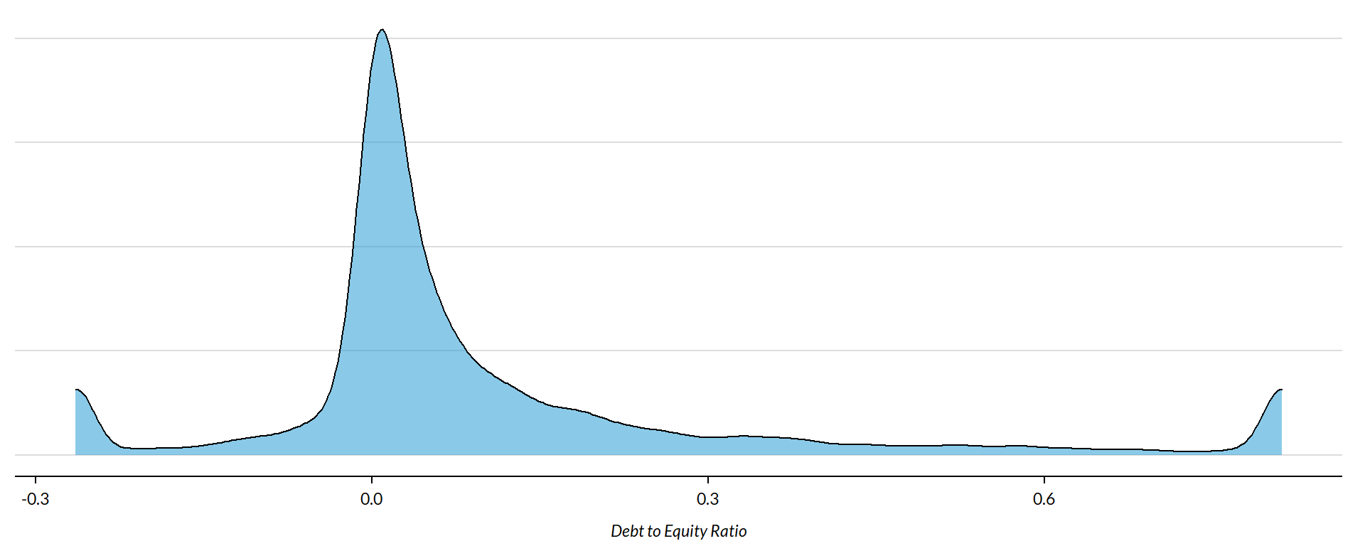
Debt/Equity Ratio by NTEE Major Code
core3 <- core2 %>% filter( ! is.na(NTEE1) )
table( core3$NTEE1) %>% sort(decreasing=TRUE) %>% kable()| Var1 | Freq |
|---|---|
| Housing | 2837 |
| Community Development | 1585 |
| Human Services | 1102 |
t <- table( factor(core3$NTEE1) )
df <- data.frame( x=Inf, y=Inf,
                  N=paste0( "N=", as.character(t) ),
                  NTEE1=names(t) )

ggplot( core3, aes( x=der ) ) +
  geom_density( alpha = 0.5) +
  # xlim( -0.1, 1 ) +
  labs( title="Nonprofit Subsectors" ) +
  xlab( variable.label ) +
  facet_wrap( ~ NTEE1, nrow=1 ) +
    theme_minimal( base_size = 15 )  +
    theme( axis.title.y=element_blank(),
           axis.text.y=element_blank(),
           axis.ticks.y=element_blank(),
           strip.text = element_text( face="bold") ) +  # size=20
  geom_text( data=df,
             aes(x, y, label=N ),
             hjust=2, vjust=3,
             color="gray60", size=6 )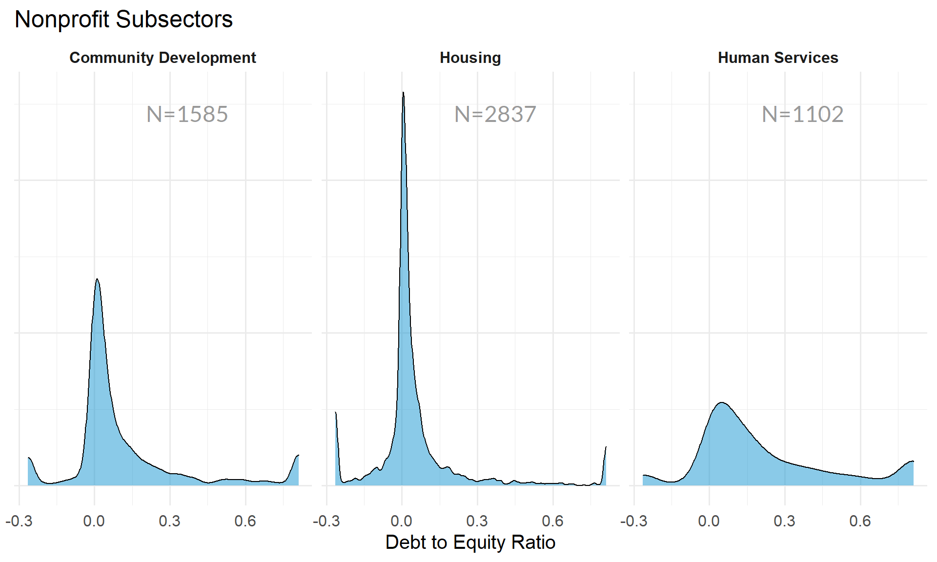
Debt/Equity Ratio by Region
table( core2$Region) %>% kable()| Var1 | Freq |
|---|---|
| Midwest | 1444 |
| Northeast | 1368 |
| South | 1610 |
| West | 1088 |
t <- table( factor(core2$Region) )
df <- data.frame( x=Inf, y=Inf,
                  N=paste0( "N=", as.character(t) ),
                  Region=names(t) )

core2 %>%
  filter( ! is.na(Region) ) %>%
  ggplot( aes(der) )  +
    geom_density( alpha = 0.5 ) +
    xlab( "Census Regions" ) +
    ylab( variable.label ) +
    facet_wrap( ~ Region, nrow=3 ) +
    theme_minimal( base_size = 22 )  +
    theme( axis.title.y=element_blank(),
           axis.text.y=element_blank(),
           axis.ticks.y=element_blank() ) +
    geom_text( data=df,
             aes(x, y, label=N ),
             hjust=2, vjust=3,
             color="gray60", size=6 )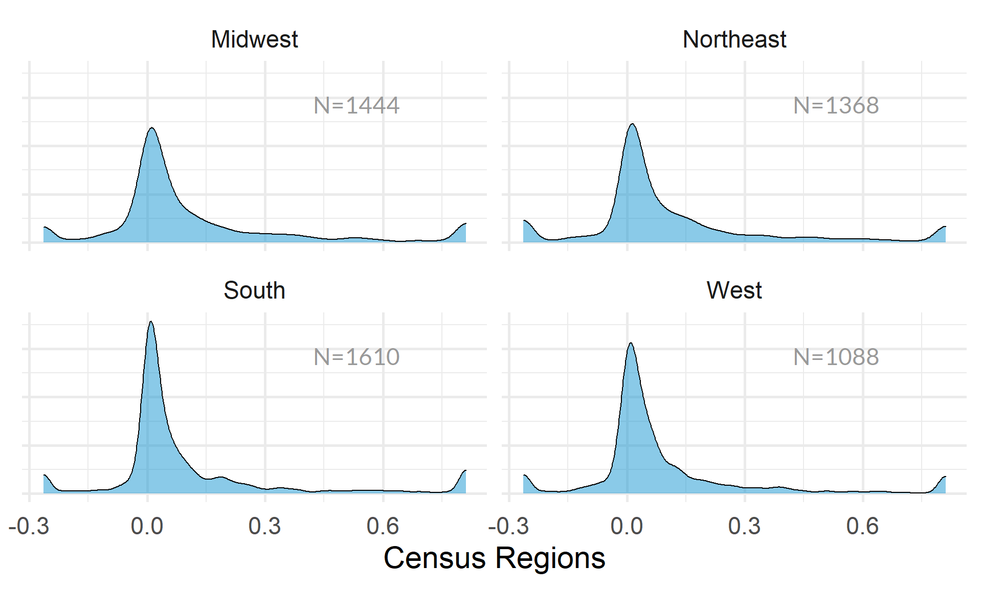
table( core2$Division ) %>% kable()| Var1 | Freq |
|---|---|
| East North Central | 1038 |
| East South Central | 289 |
| Middle Atlantic | 904 |
| Mountain | 303 |
| New England | 464 |
| Pacific | 785 |
| South Atlantic | 900 |
| West North Central | 406 |
| West South Central | 421 |
t <- table( factor(core2$Division) )
df <- data.frame( x=Inf, y=Inf,
                  N=paste0( "N=", as.character(t) ),
                  Division=names(t) )

core2 %>%
  filter( ! is.na(Division) ) %>%
  ggplot( aes(der) )  +
    geom_density( alpha = 0.5 ) +
    xlab( "Census Sub-Regions (10)" ) +
    ylab( variable.label ) +
    facet_wrap( ~ Division, nrow=3 ) +
    theme_minimal( base_size = 22 )  +
    theme( axis.title.y=element_blank(),
           axis.text.y=element_blank(),
           axis.ticks.y=element_blank() ) +
    geom_text( data=df,
             aes(x, y, label=N ),
             hjust=2, vjust=3,
color="gray60", size=6 ) 
Debt/Equity Ratio by Nonprofit Size (Expenses)
ggplot( core2, aes(x = totfuncexpns )) +
  geom_density( alpha = 0.5 ) +
  xlim( quantile(core2$totfuncexpns, c(0.02,0.98), na.rm=T ) )
core2$totfuncexpns[ core2$totfuncexpns < 1 ] <- 1
# core2$totfuncexpns[ is.na(core2$totfuncexpns) ] <- 1

if( nrow(core2) > 10000 )
{
  core3 <- sample_n( core2, 10000 )
} else
{
  core3 <- core2
}

jplot( log10(core3$totfuncexpns), core3$der,
       xlab="Nonprofit Size (logged Expenses)",
       ylab=variable.label,
       xaxt="n", xlim=c(3,10) )
axis( side=1,
      at=c(3,4,5,6,7,8,9,10),
      labels=c("1k","10k","100k","1m","10m","100m","1b","10b") )
core2 %>%
  filter( ! is.na(exp.q) ) %>%
  ggplot( aes(der) )  +
    geom_density( alpha = 0.5) +
    labs( title="Nonprofit Size (logged expenses)" ) +
    xlab( variable.label ) +
    facet_wrap( ~ exp.q, nrow=3 ) +
    theme_minimal( base_size = 22 )  +
    theme( axis.title.y=element_blank(),
           axis.text.y=element_blank(),
           axis.ticks.y=element_blank() )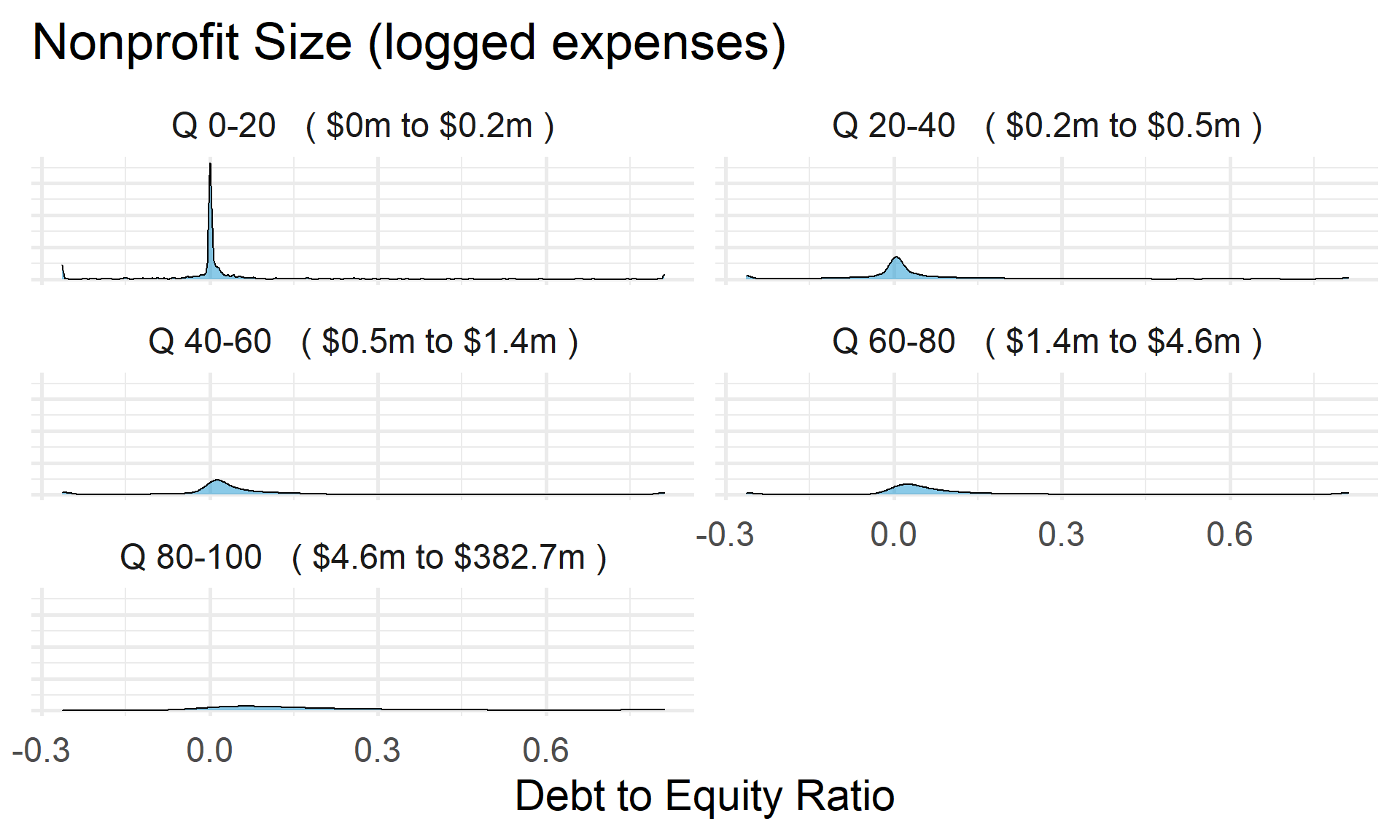
Debt/Equity Ratio by Nonprofit Size (Revenue)
ggplot( core2, aes(x = totrevenue )) +
  geom_density( alpha = 0.5 ) +
  xlim( quantile(core2$totrevenue, c(0.02,0.98), na.rm=T ) ) +
  theme( axis.title.y=element_blank(),
           axis.text.y=element_blank(),
           axis.ticks.y=element_blank() )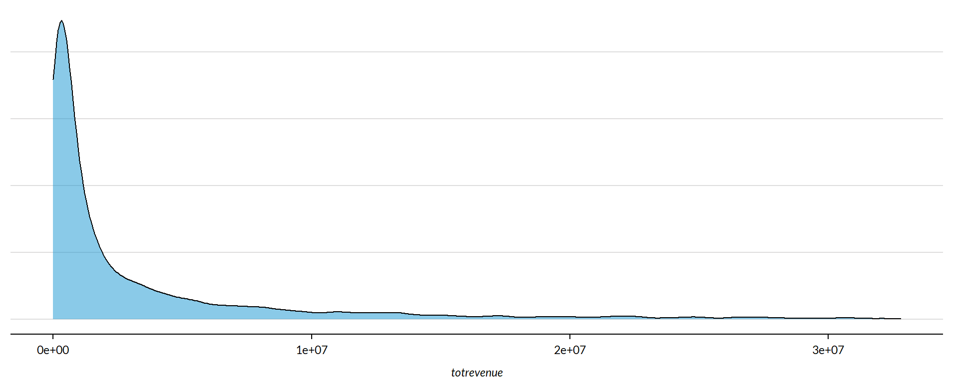
core2$totrevenue[ core2$totrevenue < 1 ] <- 1

if( nrow(core2) > 10000 )
{
  core3 <- sample_n( core2, 10000 )
} else
{
  core3 <- core2
}

jplot( log10(core3$totrevenue), core3$der,
       xlab="Nonprofit Size (logged Revenue)",
       ylab=variable.label,
       xaxt="n", xlim=c(3,10) )
axis( side=1,
      at=c(3,4,5,6,7,8,9,10),
      labels=c("1k","10k","100k","1m","10m","100m","1b","10b") )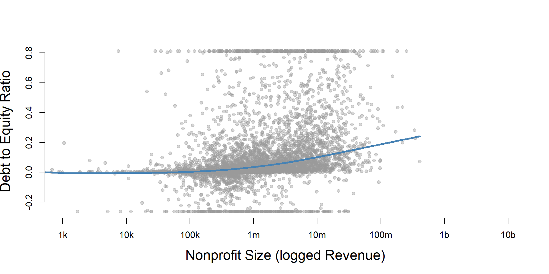
core2 %>%
  filter( ! is.na(rev.q) ) %>%
  ggplot( aes(der) )  +
    geom_density( alpha = 0.5 ) +
    labs( title="Nonprofit Size (logged revenues)" ) +
    xlab( variable.label ) +
    facet_wrap( ~ rev.q, nrow=3 ) +
    theme_minimal( base_size = 22 )  +
    theme( axis.title.y=element_blank(),
           axis.text.y=element_blank(),
           axis.ticks.y=element_blank() )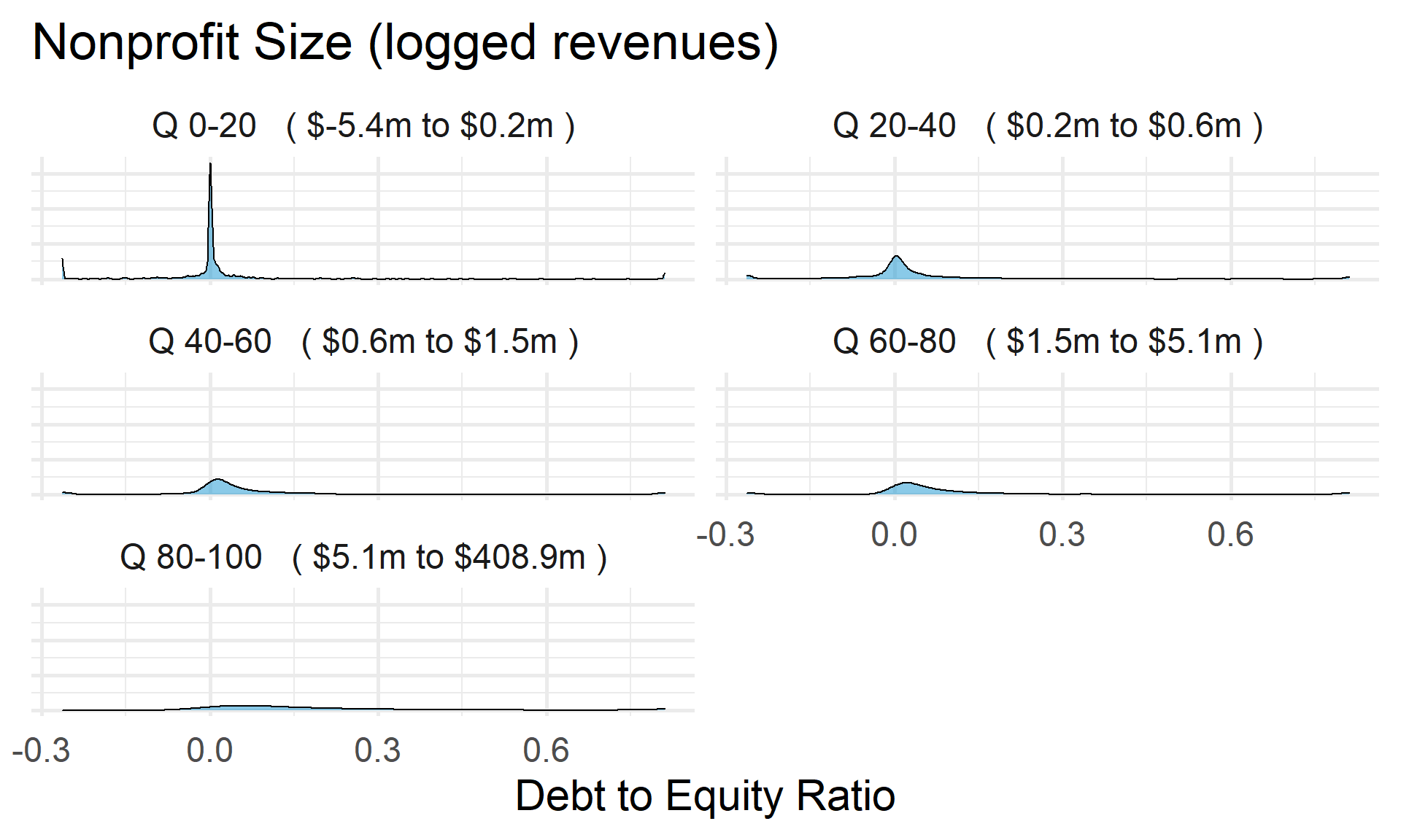
Debt/Equity Ratio by Nonprofit Size (Net Assets)
ggplot( core2, aes(x = totnetassetend )) +
  geom_density( alpha = 0.5) +
  xlim( quantile(core2$totnetassetend, c(0.02,0.98), na.rm=T ) ) +
  xlab( "Net Assets" ) +
    theme( axis.title.y=element_blank(),
           axis.text.y=element_blank(),
           axis.ticks.y=element_blank() )
core2$totnetassetend[ core2$totnetassetend < 1 ] <- NA

if( nrow(core2) > 10000 )
{
  core3 <- sample_n( core2, 10000 )
} else
{
  core3 <- core2
}

jplot( log10(core3$totnetassetend), core3$der,
       xlab="Nonprofit Size (logged Net Assets)",
       ylab=variable.label,
       xaxt="n", xlim=c(3,10) )
axis( side=1,
      at=c(3,4,5,6,7,8,9,10),
      labels=c("1k","10k","100k","1m","10m","100m","1b","10b") )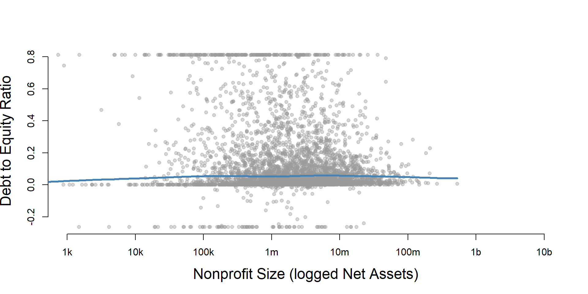
core2$totnetassetend[ core2$totnetassetend < 1 ] <- NA
core2$asset.q <- create_quantiles( var=core2$totnetassetend, n.groups=5 )

core2 %>%
  filter( ! is.na(asset.q) ) %>%
  ggplot( aes(der) )  +
    geom_density( alpha = 0.5 ) +
    labs( title="Nonprofit Size (logged net assets, if assets > 0)" ) +
    xlab( variable.label ) +
    ylab( "" ) +
    facet_wrap( ~ asset.q, nrow=3 ) +
    theme_minimal( base_size = 22 )  +
    theme( axis.title.y=element_blank(),
           axis.text.y=element_blank(),
           axis.ticks.y=element_blank() )
Total Assets for Comparison
core2$totassetsend[ core2$totassetsend < 1 ] <- NA
core2$tot.asset.q <- create_quantiles( var=core2$totassetsend, n.groups=5 )

if( nrow(core2) > 10000 )
{
  core3 <- sample_n( core2, 10000 )
} else
{
  core3 <- core2
}

jplot( log10(core3$totassetsend), core3$der,
       xlab="Nonprofit Size (logged Total Assets)",
       ylab=variable.label,
       xaxt="n", xlim=c(3,10) )
axis( side=1,
      at=c(3,4,5,6,7,8,9,10),
      labels=c("1k","10k","100k","1m","10m","100m","1b","10b") )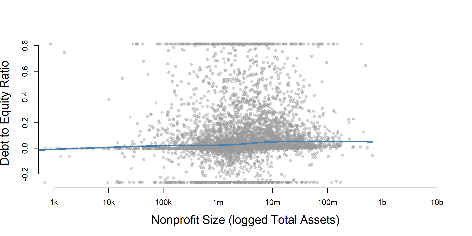
ggplot( core2, aes(x = totassetsend )) +
  geom_density( alpha = 0.5) +
  xlim( quantile(core2$totassetsend, c(0.02,0.98), na.rm=T ) ) +
  xlab( "Net Assets" ) +
    theme( axis.title.y=element_blank(),
           axis.text.y=element_blank(),
           axis.ticks.y=element_blank() )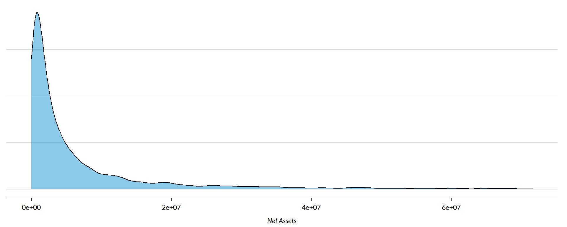
core2 %>%
  filter( ! is.na(tot.asset.q) ) %>%
  ggplot( aes(der) )  +
    geom_density( alpha = 0.5 ) +
    xlab( "Nonprofit Size (logged total assets, if assets > 0)" ) +
    ylab( variable.label ) +
    facet_wrap( ~ tot.asset.q, nrow=3 ) +
    theme_minimal( base_size = 22 )  +
    theme( axis.title.y=element_blank(),
           axis.text.y=element_blank(),
           axis.ticks.y=element_blank() )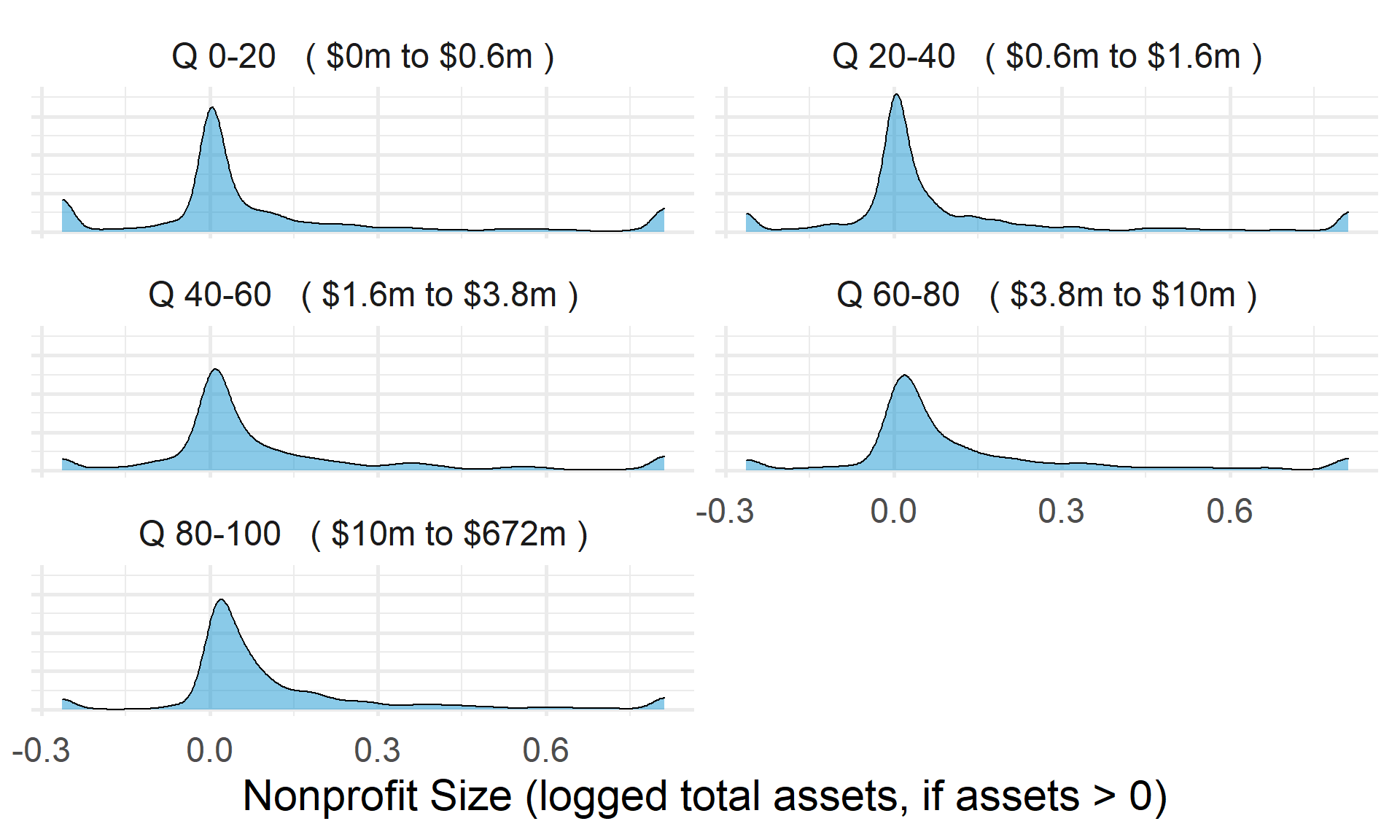
Debt/Equity Ratio by Nonprofit Age
ggplot( core2, aes(x = AGE )) +
geom_density( alpha = 0.5 ) 
core2$AGE[ core2$AGE < 1 ] <- NA

if( nrow(core2) > 10000 )
{
  core3 <- sample_n( core2, 10000 )
} else
{
  core3 <- core2
}

jplot( core3$AGE, core3$der,
       xlab="Nonprofit Age",
ylab=variable.label ) 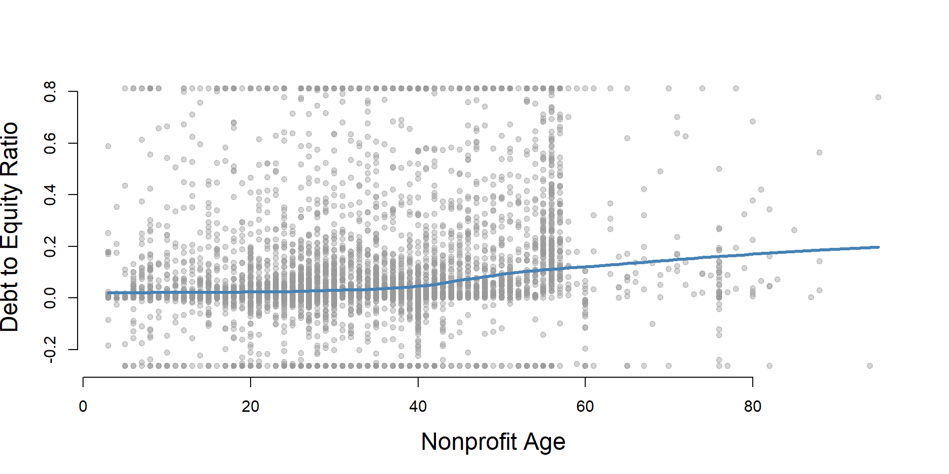
core2 %>%
  filter( ! is.na(age.q) ) %>%
  ggplot( aes(der) )  +
    geom_density( alpha = 0.5 ) +
    labs( title="Nonprofit Age" ) +
    xlab( variable.label ) +
    ylab( "" ) +
    facet_wrap( ~ age.q, nrow=3 ) +
    theme_minimal( base_size = 22 )  +
    theme( axis.title.y=element_blank(),
           axis.text.y=element_blank(),
           axis.ticks.y=element_blank() )
Debt/Equity Ratio by Land and Building Value
ggplot( core2, aes(x = lndbldgsequipend )) +
geom_density( alpha = 0.5 ) 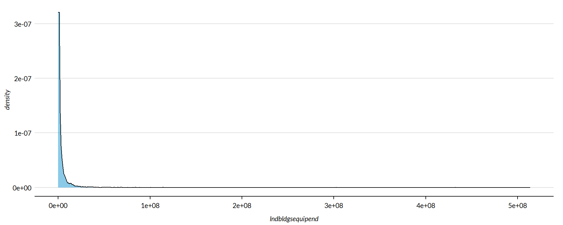
core2$lndbldgsequipend[ core2$lndbldgsequipend < 1 ] <- NA
if( nrow(core2) > 10000 )
{
  core3 <- sample_n( core2, 10000 )
} else
{
  core3 <- core2


jplot( log10(core3$lndbldgsequipend), core3$dar,
       xlab="Land and Building Value (logged)",
       ylab=variable.label,
       xaxt="n", xlim=c(3,10) )
axis( side=1,
      at=c(3,4,5,6,7,8,9,10),
      labels=c("1k","10k","100k","1m","10m","100m","1b","10b") )
}
## Error in lowess(x2[ok] ~ x1[ok]): invalid input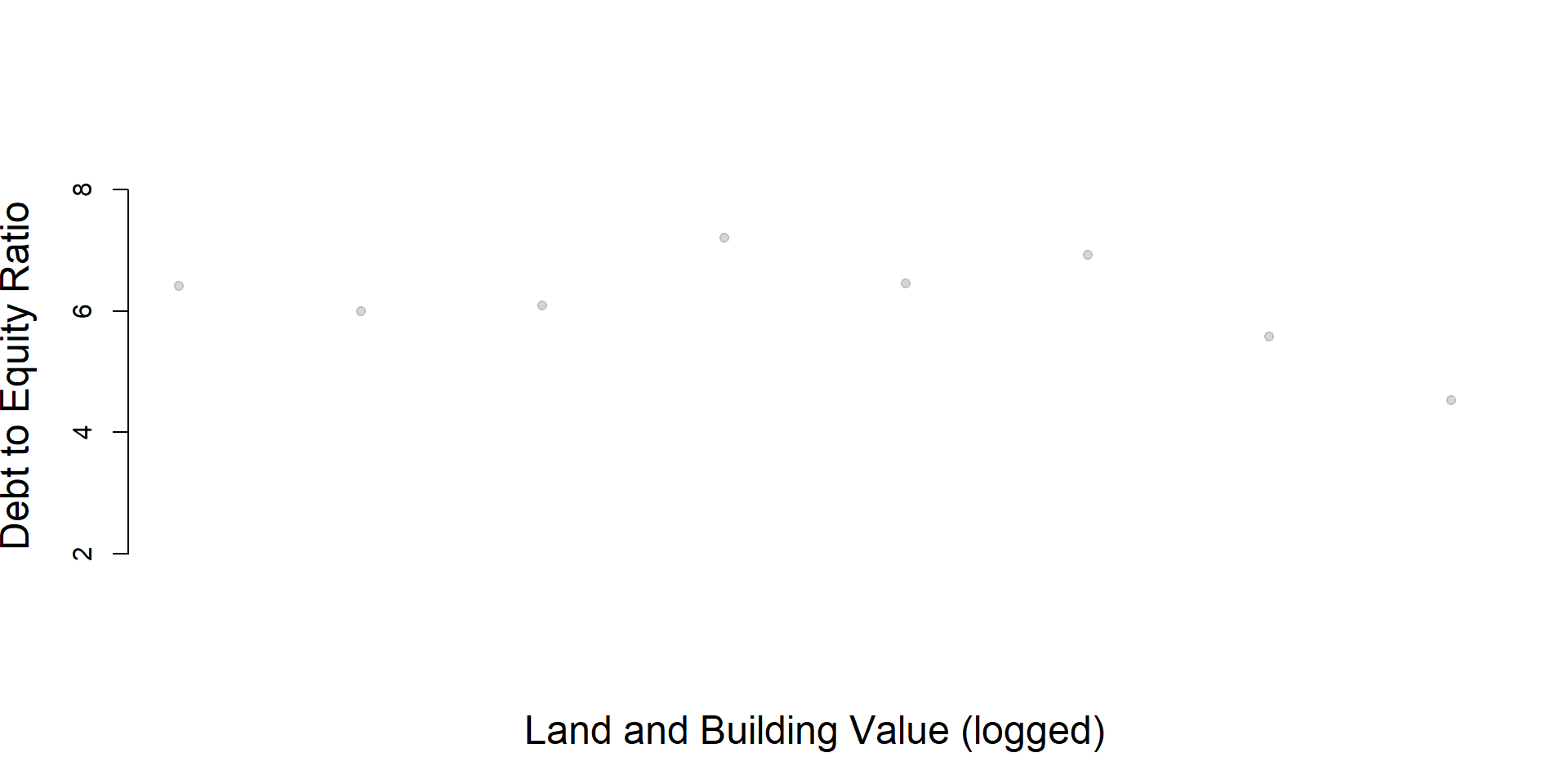
core2 %>%
  filter( ! is.na(land.q) ) %>%
  ggplot( aes(dar) )  +
    geom_density( alpha = 0.5 ) +
    labs( title="Land and Building Value" ) +
    xlab( variable.label ) +
    ylab( "" ) +
    facet_wrap( ~ land.q, nrow=3 ) +
    theme_minimal( base_size = 22 )  +
    theme( axis.title.y=element_blank(),
           axis.text.y=element_blank(),
           axis.ticks.y=element_blank() )
## Error in FUN(X[[i]], ...): object 'dar' not found
Save Metrics
core.der <- select( core, ein, tax_pd, der )
saveRDS( core.der, "03-data-ratios/m-04-debt-equity-ratio.rds" )
write.csv( core.der, "03-data-ratios/m-04-debt-equity-ratio.csv" )