Metric 07- Land to Assets Ratio
April 8, 2022
## Error in local:core <- readRDS("02-data-wrangled/core.rds"): could not find function ":<-"![]()
Metric Construction
Definition & Interpretation
\[Land \: and \: Buildings \: to \: Assets \: Ratio = \frac{Land \: and \: Buildings}{Total \: Assets} \]
This metric shows the proportion of an organization’s total assets that are made up by land and buildings. It shows how diversified their asset portfolio is and somewhat how specialized their line of work is within housing or building development.
Higher values mean that an organization has more of its asset portfolio in land and buildings, and lower values mean that development or land and building holdings represent a small share of what the organization’s activities and finances are tied up in.
Variables
Note: This data is available only for organizations that file full 990s. [Organizations with revenues <$200,000 and total assets <$500,000 have the option to not file a full 990 and file an EZ instead.]
Numerator: Land, buildings, and equipment (net of
depreciation) EOY
On 990: Part X, line 10B
SOI PC EXTRACTS: lndbldgsequipend
On EZ:Not available
Denominator: Total AssetsOn 990: Part X, Line 16B -SOI PC EXTRACTS: totassetsend
On EZ: Part II, line 25B -SOI PC EXTRACTS: totassetsend
# TEMPORARY VARIABLES
landvalue  <- ( core$lndbldgsequipend)
assets <- ( core$totassetsend)

# can't divide by zero
assets[ assets == 0 ] <- NA

# SAVE RESULTS
core$lb_to_assets <-  landvalue / assets

# summary( core$lb_to_assets )
Standardize Scales
Check high and low values to see what makes sense.
x.05 <- quantile( core$lb_to_assets, 0.05, na.rm=T )
x.95 <- quantile( core$lb_to_assets, 0.95, na.rm=T )

ggplot( core, aes(x = lb_to_assets ) ) +
  geom_density( alpha = 0.5) +
xlim( x.05, x.95 ) 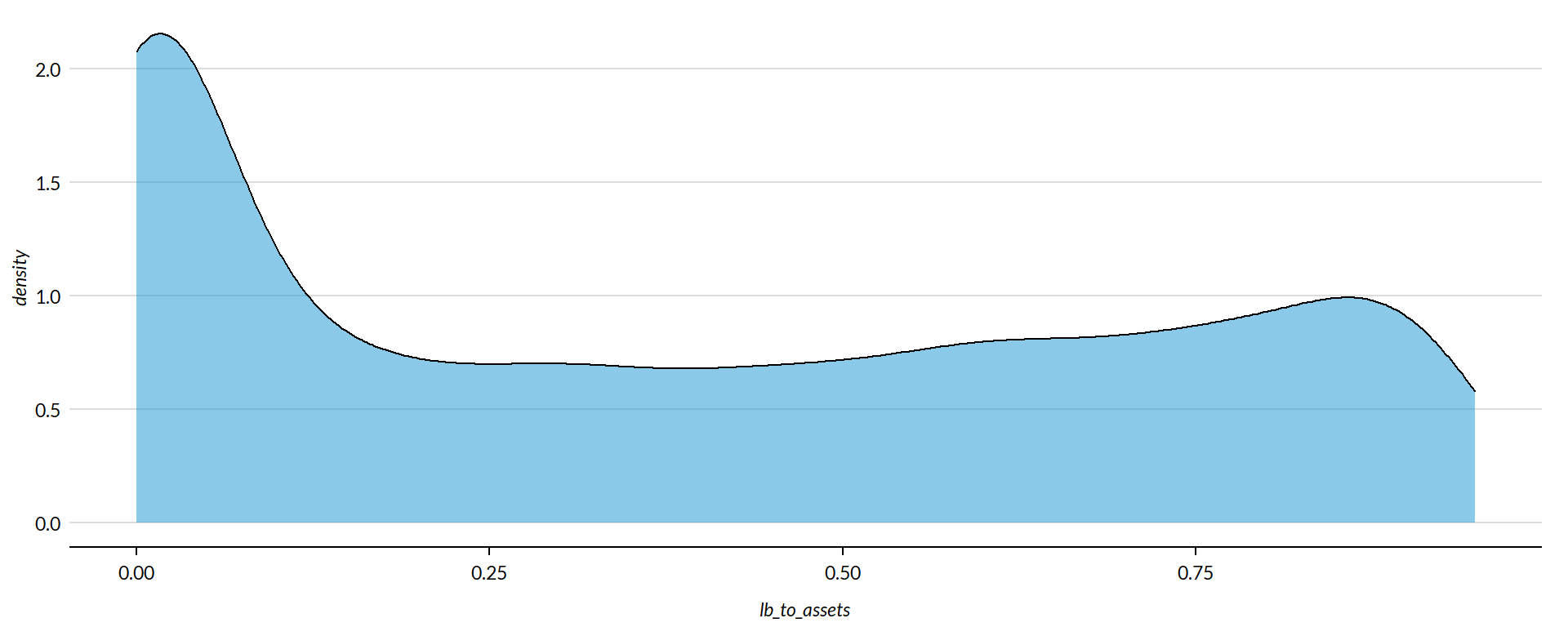
Winsorization: All extreme values have been capped by replacing any values below the 5% distribution and above the 95% distribution with the 5% and 95% values. Consequently the end tails to all density charts may be slightly higher than reality but the visuals will be scaled for better viewing (not skewed by outliers).
core2 <- core

# proportion of values that are negative
mean( core2$lb_to_assets < 0, na.rm=T )
## [1] 0.0001884304
core2$lb_to_assets[ core2$lb_to_assets < 0 ] <- 0

# proption of values above 200%
mean( core2$lb_to_assets > 50, na.rm=T )
## [1] 0.0001884304
core2$lb_to_assets[ core2$lb_to_assets > 50 ] <- 50


x.05 <- quantile( core$lb_to_assets, 0.05, na.rm=T )
x.95 <- quantile( core$lb_to_assets, 0.95, na.rm=T )

core2 <- core

# proportion of values that are negative
# mean( core2$der < 0, na.rm=T )

# proption of values above 1%
# mean( core2$der > 5, na.rm=T )

# WINSORIZATION AT 5th and 95th PERCENTILES

core2$lb_to_assets[ core2$lb_to_assets < x.05 ] <- x.05
core2$lb_to_assets[ core2$lb_to_assets > x.95 ] <- x.95
Metric Scope
Tax data is available for full 990 filers, so this metric does not describe any organizations with Gross receipts < $200,000 and Total assets < $500,000. Some organizations with receipts or assets below those thresholds may have filed a full 990, but these would be exceptions.
The data have been capped to those with values between 5% and 95% of the normal distribution to cut off outliers and non-land-value-holding organizations.
Descriptive Statistics
Convert all monetary variables to thousands of dollars.
core2 %>%
  mutate( lb_to_assets = lb_to_assets * 100,
    totrevenue = totrevenue / 1000,
    totfuncexpns = totfuncexpns / 1000,
    lndbldgsequipend = lndbldgsequipend / 1000,
    totassetsend = totassetsend / 1000,
    totliabend = totliabend / 1000,
    totnetassetend = totnetassetend / 1000 ) %>%
  select( STATE,  NTEE1, NTMAJ12,
          lb_to_assets,
          AGE,
          totrevenue, totfuncexpns,
          lndbldgsequipend, totassetsend,
          totnetassetend, totliabend ) %>%

  stargazer( type = s.type,
             digits=0,
             summary.stat = c("min","p25","median",
                              "mean","p75","max", "sd"),
             covariate.labels = c("Land to Assets Ratio*", "Age",
                                  "Revenue ($1k)", "Expenses($1k)",
                                  "Buildings ($1k)", "Total Assets ($1k)",
"Net Assets ($1k)", "Liabiliies ($1k)"))| Statistic | Min | Pctl(25) | Median | Mean | Pctl(75) | Max | St. Dev. |
| Land to Assets Ratio* | 0 | 5 | 39 | 42 | 74 | 95 | 34 |
| Age | 3 | 22 | 30 | 32 | 41 | 95 | 15 |
| Revenue (1k) | -5,377 | 259 | 909 | 4,522 | 3,672 | 408,932 | 14,286 |
| Expenses(1k) | 0 | 263 | 840 | 4,192 | 3,328 | 382,667 | 13,466 |
| Buildings (1k) | -4 | 79 | 824 | 3,504 | 2,868 | 513,509 | 13,210 |
| Total Assets (1k) | -7,552 | 778 | 2,446 | 9,262 | 7,477 | 672,021 | 27,039 |
| Net Assets (1k) | -178,870 | 156 | 1,094 | 4,553 | 4,079 | 531,068 | 15,470 |
| Liabiliies (1k) | -2,707 | 115 | 816 | 4,709 | 3,133 | 705,623 | 18,722 |
*Note: The Land to Assets Ratio is usually a 0 to 1 ratio but has been scaled by 100 in this descriptive table for better readability.
What proportion of orgs have land and building asset values
equal to zero?
prop.zero <- mean( core2$lb_to_assets == 0, na.rm=T )In the sample, 12 percent of the organizations land and building asset values equal to zero. These organizations are dropped from subsequent graphs to keep the visualizations clean. The interpretation of the graphics should be the distributions of land and buildings to assets ratio for organizations that have some land and buildings.
###
### ADD QUANTILES
###
###   function create_quantiles() defined in r-functions.R

core2$exp.q   <- create_quantiles( var=core2$totfuncexpns,   n.groups=5 )
core2$rev.q   <- create_quantiles( var=core2$totrevenue,     n.groups=5 )
core2$asset.q <- create_quantiles( var=core2$totnetassetend, n.groups=5 )
core2$age.q   <- create_quantiles( var=core2$AGE,            n.groups=5 )
core2$land.q  <- create_quantiles( var=core2$lndbldgsequipend,      n.groups=5 )
Land and Building Share Density
min.x <- min( core2$lb_to_assets, na.rm=T )
max.x <- max( core2$lb_to_assets, na.rm=T )

ggplot( core2, aes(x = lb_to_assets )) +
  geom_density( alpha = 0.5 ) +
  xlim( min.x, max.x  ) +
  xlab( variable.label ) +
  theme( axis.title.y=element_blank(),
         axis.text.y=element_blank(),
         axis.ticks.y=element_blank() )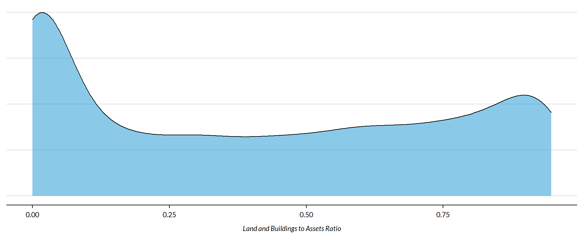
Land and Building Share by NTEE Major Code
core3 <- core2 %>% filter( ! is.na(NTEE1) )
table( core3$NTEE1) %>% sort(decreasing=TRUE) %>% kable()| Var1 | Freq |
|---|---|
| Housing | 2837 |
| Community Development | 1585 |
| Human Services | 1102 |
t <- table( factor(core3$NTEE1) )
df <- data.frame( x=Inf, y=Inf,
                  N=paste0( "N=", as.character(t) ),
                  NTEE1=names(t) )

ggplot( core3, aes( x=lb_to_assets ) ) +
  geom_density( alpha = 0.5) +
  # xlim( -0.1, 1 ) +
  labs( title="Nonprofit Subsectors" ) +
  xlab( variable.label ) +
  facet_wrap( ~ NTEE1, nrow=1 ) +
    theme_minimal( base_size = 15 )  +
    theme( axis.title.y=element_blank(),
           axis.text.y=element_blank(),
           axis.ticks.y=element_blank(),
           strip.text = element_text( face="bold") ) +  # size=20
  geom_text( data=df,
             aes(x, y, label=N ),
             hjust=2, vjust=3,
             color="gray60", size=6 )
Land and Building Share by Region
table( core2$Region) %>% kable()| Var1 | Freq |
|---|---|
| Midwest | 1444 |
| Northeast | 1368 |
| South | 1610 |
| West | 1088 |
t <- table( factor(core2$Region) )
df <- data.frame( x=Inf, y=Inf,
                  N=paste0( "N=", as.character(t) ),
                  Region=names(t) )

core2 %>%
  filter( ! is.na(Region) ) %>%
  ggplot( aes(lb_to_assets) )  +
    geom_density( alpha = 0.5 ) +
    xlab( "Census Regions" ) +
    ylab( variable.label ) +
    facet_wrap( ~ Region, nrow=3 ) +
    theme_minimal( base_size = 22 )  +
    theme( axis.title.y=element_blank(),
           axis.text.y=element_blank(),
           axis.ticks.y=element_blank() ) +
    geom_text( data=df,
             aes(x, y, label=N ),
             hjust=2, vjust=3,
             color="gray60", size=6 )
table( core2$Division ) %>% kable()| Var1 | Freq |
|---|---|
| East North Central | 1038 |
| East South Central | 289 |
| Middle Atlantic | 904 |
| Mountain | 303 |
| New England | 464 |
| Pacific | 785 |
| South Atlantic | 900 |
| West North Central | 406 |
| West South Central | 421 |
t <- table( factor(core2$Division) )
df <- data.frame( x=Inf, y=Inf,
                  N=paste0( "N=", as.character(t) ),
                  Division=names(t) )

core2 %>%
  filter( ! is.na(Division) ) %>%
  ggplot( aes(lb_to_assets) )  +
    geom_density( alpha = 0.5 ) +
    xlab( "Census Sub-Regions (10)" ) +
    ylab( variable.label ) +
    facet_wrap( ~ Division, nrow=3 ) +
    theme_minimal( base_size = 22 )  +
    theme( axis.title.y=element_blank(),
           axis.text.y=element_blank(),
           axis.ticks.y=element_blank() ) +
    geom_text( data=df,
             aes(x, y, label=N ),
             hjust=2, vjust=3,
color="gray60", size=6 ) 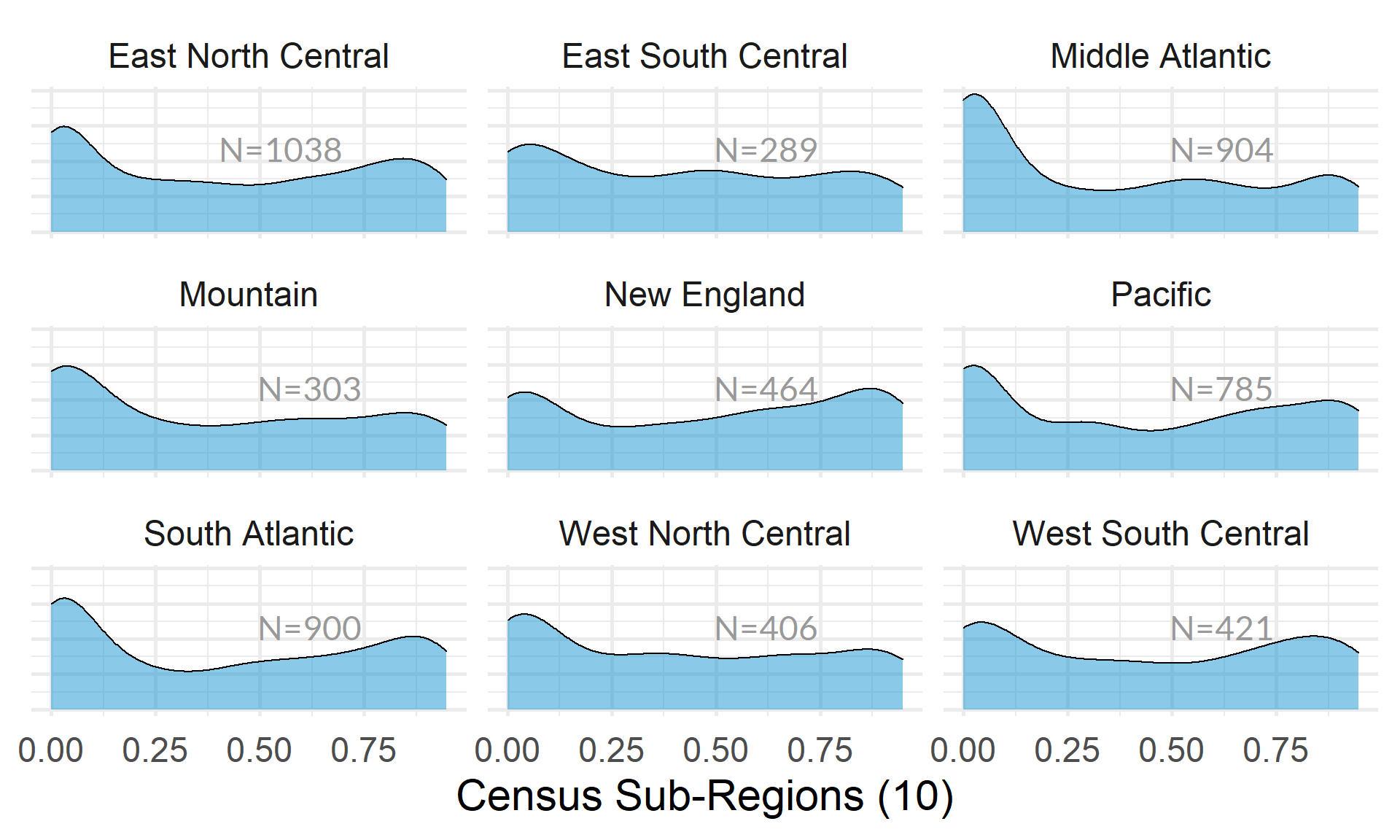
Land and Building Share by Nonprofit Size (Expenses)
ggplot( core2, aes(x = totfuncexpns )) +
  geom_density( alpha = 0.5 ) +
  xlim( quantile(core2$totfuncexpns, c(0.02,0.98), na.rm=T ) )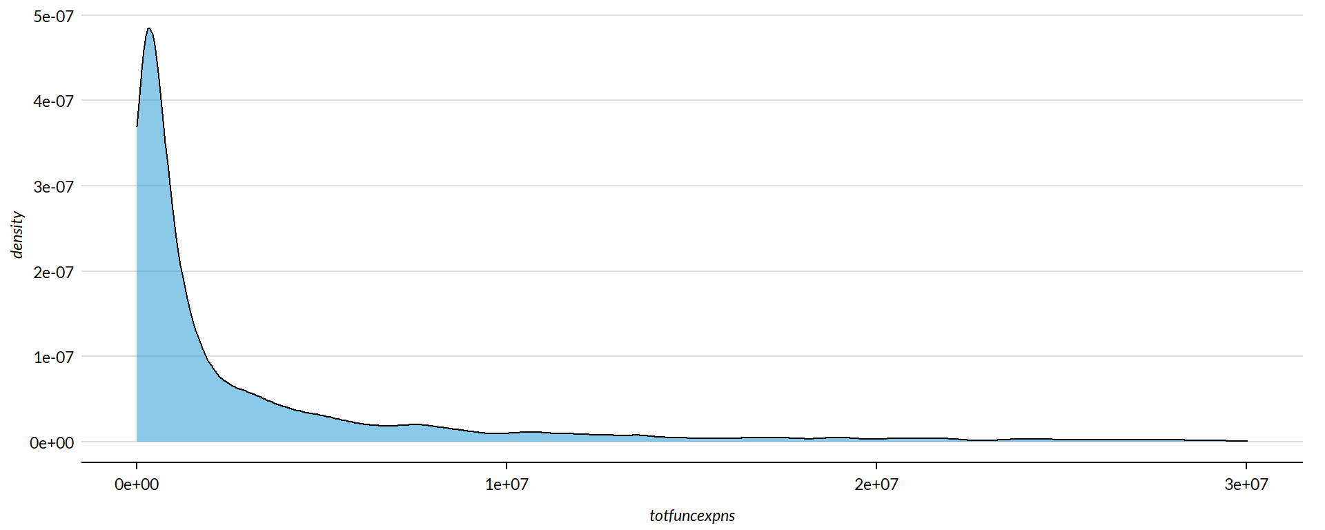
core2$totfuncexpns[ core2$totfuncexpns < 1 ] <- 1
# core2$totfuncexpns[ is.na(core2$totfuncexpns) ] <- 1

if( nrow(core2) > 10000 )
{
  core3 <- sample_n( core2, 10000 )
} else
{
  core3 <- core2
}

jplot( log10(core3$totfuncexpns), core3$lb_to_assets,
       xlab="Nonprofit Size (logged Expenses)",
       ylab=variable.label,
       xaxt="n", xlim=c(3,10) )
axis( side=1,
      at=c(3,4,5,6,7,8,9,10),
      labels=c("1k","10k","100k","1m","10m","100m","1b","10b") )
core2 %>%
  filter( ! is.na(exp.q) ) %>%
  ggplot( aes(lb_to_assets) )  +
    geom_density( alpha = 0.5) +
    labs( title="Nonprofit Size (logged expenses)" ) +
    xlab( variable.label ) +
    facet_wrap( ~ exp.q, nrow=3 ) +
    theme_minimal( base_size = 22 )  +
    theme( axis.title.y=element_blank(),
           axis.text.y=element_blank(),
           axis.ticks.y=element_blank() )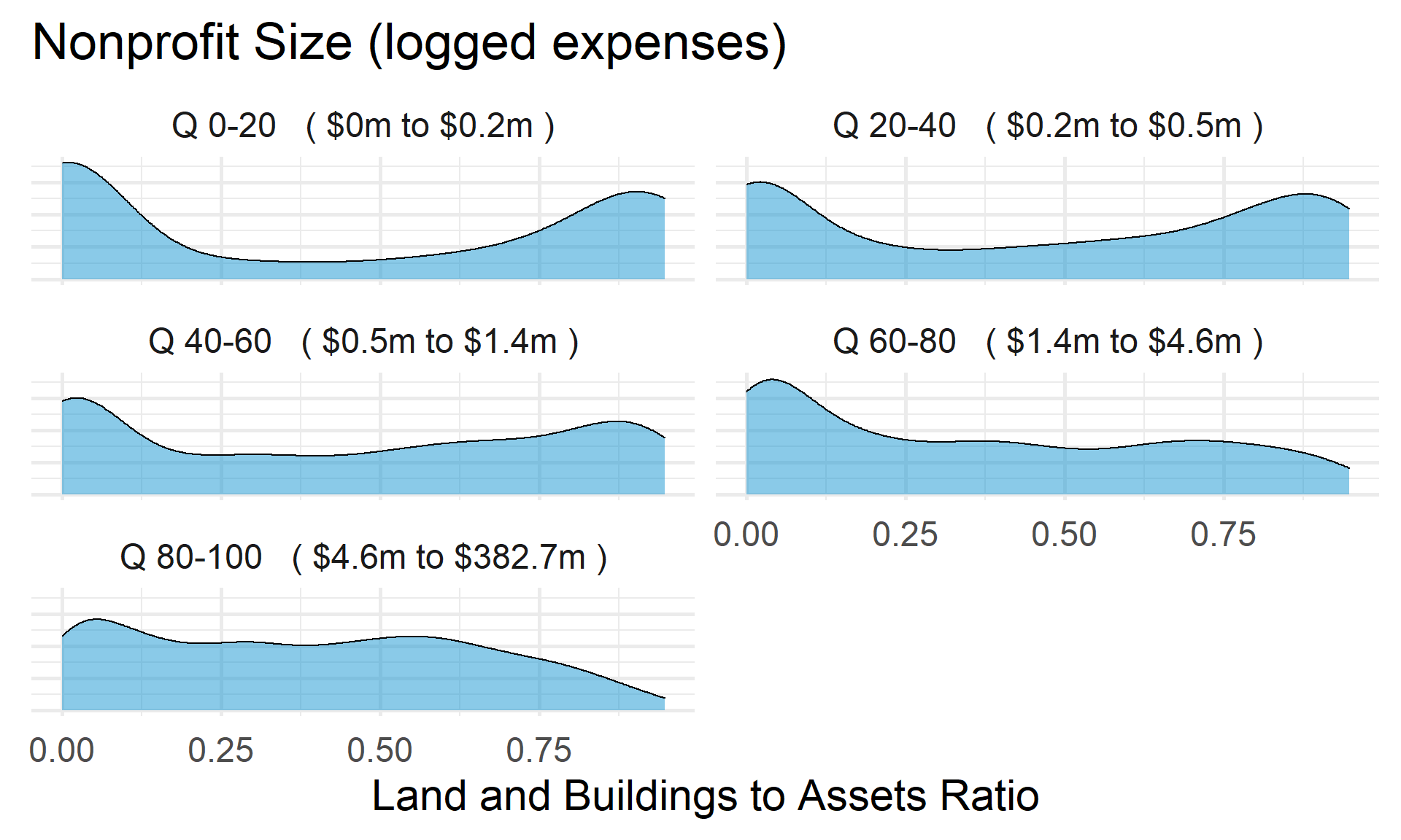
Land and Building Share by Nonprofit Size (Revenue)
ggplot( core2, aes(x = totrevenue )) +
  geom_density( alpha = 0.5 ) +
  xlim( quantile(core2$totrevenue, c(0.02,0.98), na.rm=T ) ) +
  theme( axis.title.y=element_blank(),
           axis.text.y=element_blank(),
           axis.ticks.y=element_blank() )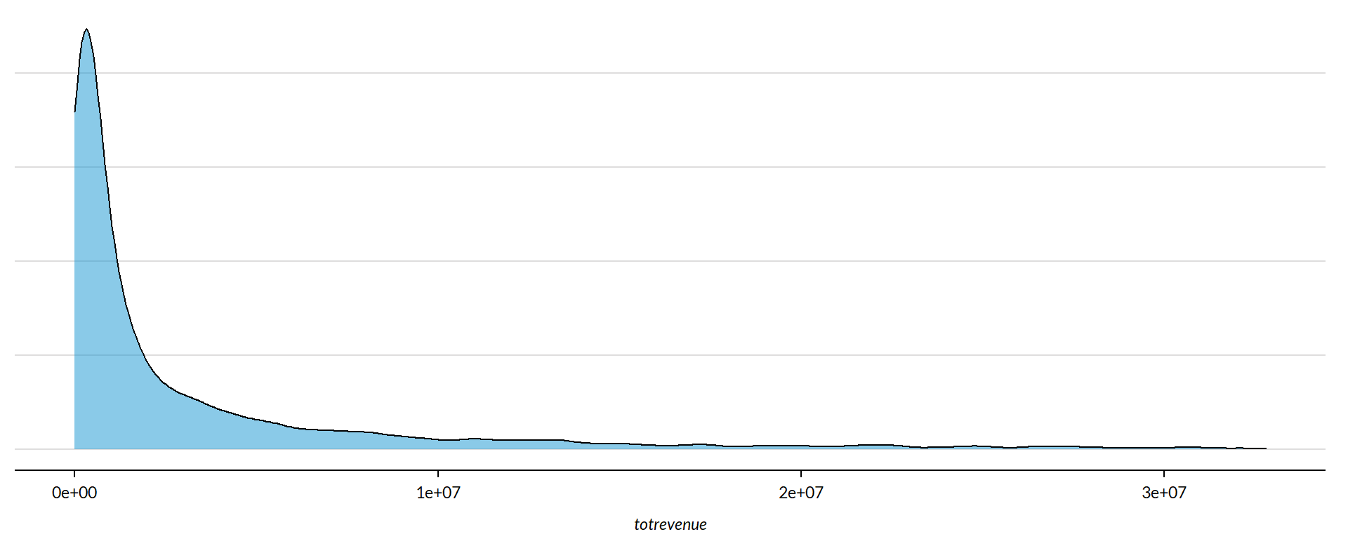
core2$totrevenue[ core2$totrevenue < 1 ] <- 1

if( nrow(core2) > 10000 )
{
  core3 <- sample_n( core2, 10000 )
} else
{
  core3 <- core2
}

jplot( log10(core3$totrevenue), core3$lb_to_assets,
       xlab="Nonprofit Size (logged Revenue)",
       ylab=variable.label,
       xaxt="n", xlim=c(3,10) )
axis( side=1,
      at=c(3,4,5,6,7,8,9,10),
      labels=c("1k","10k","100k","1m","10m","100m","1b","10b") )
core2 %>%
  filter( ! is.na(rev.q) ) %>%
  ggplot( aes(lb_to_assets) )  +
    geom_density( alpha = 0.5 ) +
    labs( title="Nonprofit Size (logged revenues)" ) +
    xlab( variable.label ) +
    facet_wrap( ~ rev.q, nrow=3 ) +
    theme_minimal( base_size = 22 )  +
    theme( axis.title.y=element_blank(),
           axis.text.y=element_blank(),
           axis.ticks.y=element_blank() )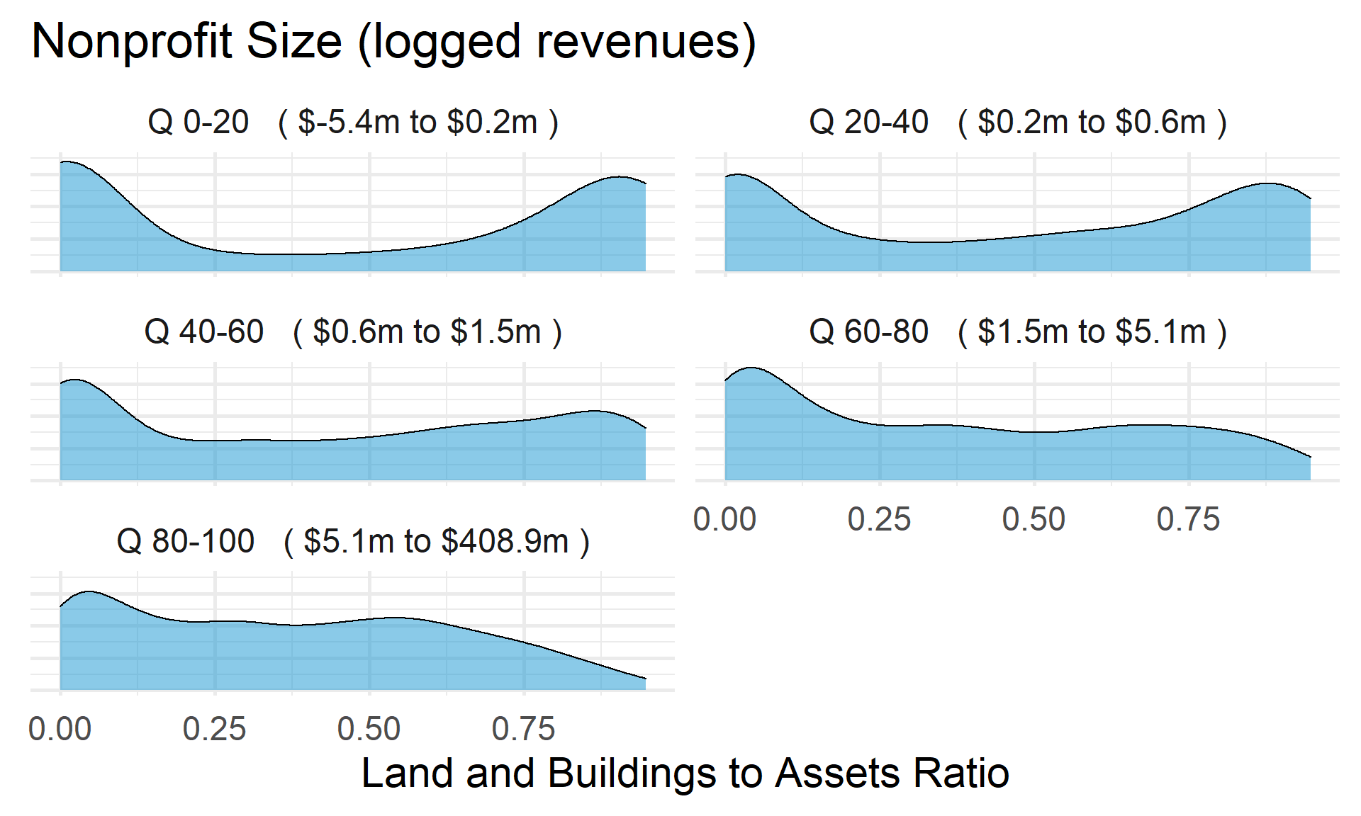
Land and Building Share by Nonprofit Size (Net Assets)
ggplot( core2, aes(x = totnetassetend )) +
  geom_density( alpha = 0.5) +
  xlim( quantile(core2$totnetassetend, c(0.02,0.98), na.rm=T ) ) +
  xlab( "Net Assets" ) +
    theme( axis.title.y=element_blank(),
           axis.text.y=element_blank(),
           axis.ticks.y=element_blank() )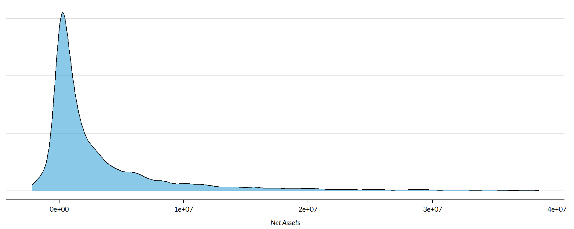
core2$totnetassetend[ core2$totnetassetend < 1 ] <- NA

if( nrow(core2) > 10000 )
{
  core3 <- sample_n( core2, 10000 )
} else
{
  core3 <- core2
}

jplot( log10(core3$totnetassetend), core3$lb_to_assets,
       xlab="Nonprofit Size (logged Net Assets)",
       ylab=variable.label,
       xaxt="n", xlim=c(3,10) )
axis( side=1,
      at=c(3,4,5,6,7,8,9,10),
      labels=c("1k","10k","100k","1m","10m","100m","1b","10b") )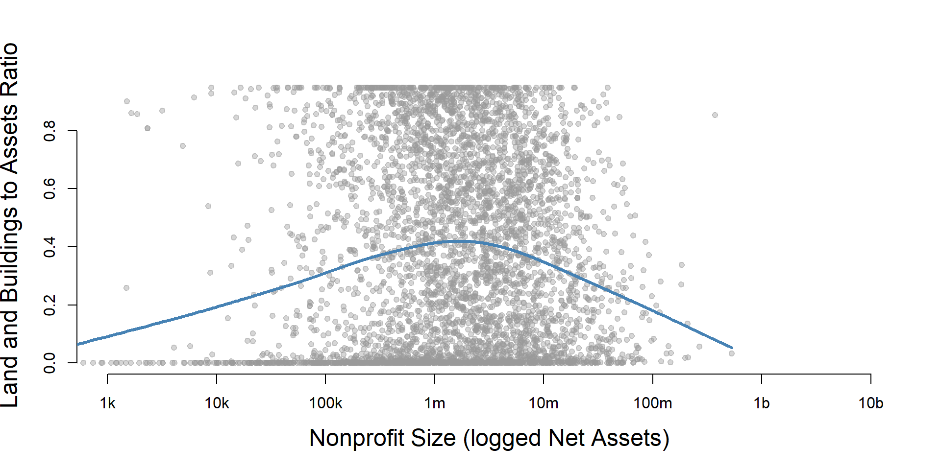
core2$totnetassetend[ core2$totnetassetend < 1 ] <- NA
core2$asset.q <- create_quantiles( var=core2$totnetassetend, n.groups=5 )

core2 %>%
  filter( ! is.na(asset.q) ) %>%
  ggplot( aes(lb_to_assets) )  +
    geom_density( alpha = 0.5 ) +
    labs( title="Nonprofit Size (logged net assets, if assets > 0)" ) +
    xlab( variable.label ) +
    ylab( "" ) +
    facet_wrap( ~ asset.q, nrow=3 ) +
    theme_minimal( base_size = 22 )  +
    theme( axis.title.y=element_blank(),
           axis.text.y=element_blank(),
           axis.ticks.y=element_blank() )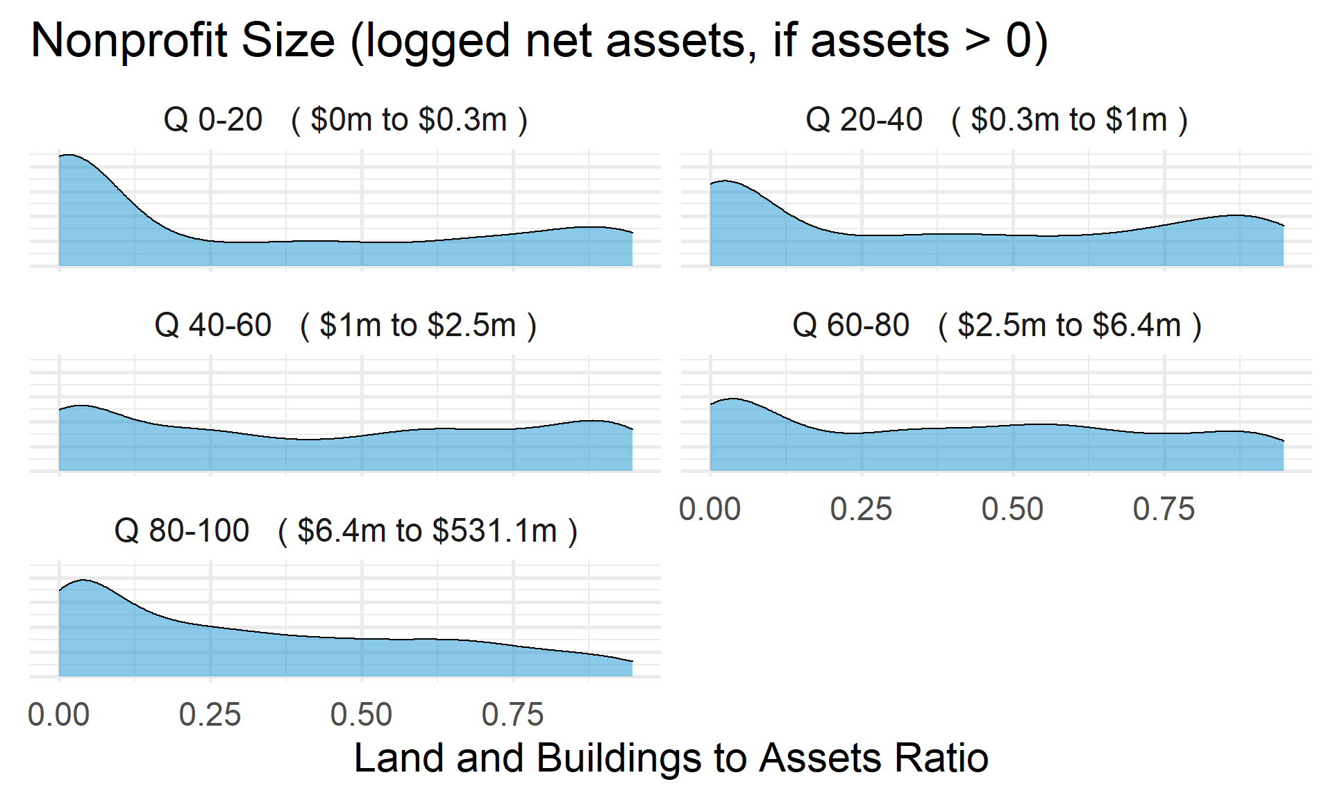
Total Assets for Comparison
core2$totassetsend[ core2$totassetsend < 1 ] <- NA
core2$tot.asset.q <- create_quantiles( var=core2$totassetsend, n.groups=5 )

if( nrow(core2) > 10000 )
{
  core3 <- sample_n( core2, 10000 )
} else
{
  core3 <- core2
}

jplot( log10(core3$totassetsend), core3$lb_to_assets,
       xlab="Nonprofit Size (logged Total Assets)",
       ylab=variable.label,
       xaxt="n", xlim=c(3,10) )
axis( side=1,
      at=c(3,4,5,6,7,8,9,10),
      labels=c("1k","10k","100k","1m","10m","100m","1b","10b") )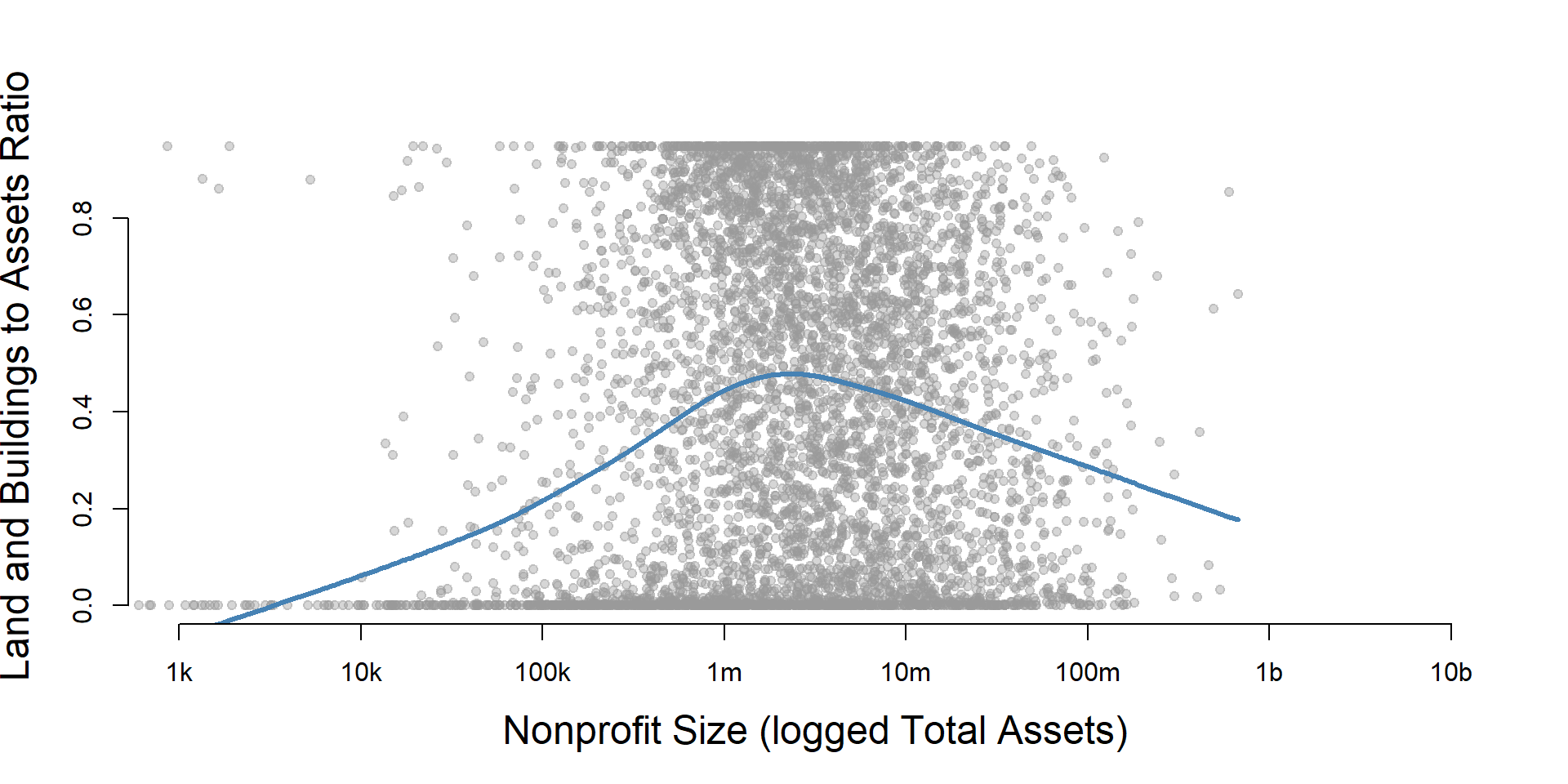
ggplot( core2, aes(x = totassetsend )) +
  geom_density( alpha = 0.5) +
  xlim( quantile(core2$totassetsend, c(0.02,0.98), na.rm=T ) ) +
  xlab( "Net Assets" ) +
    theme( axis.title.y=element_blank(),
           axis.text.y=element_blank(),
           axis.ticks.y=element_blank() )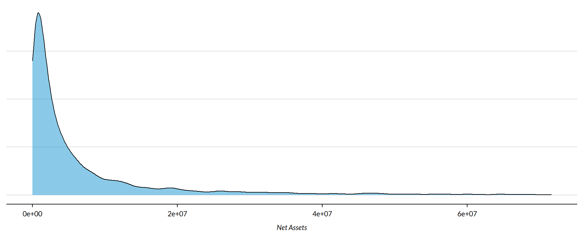
core2 %>%
  filter( ! is.na(tot.asset.q) ) %>%
  ggplot( aes(lb_to_assets) )  +
    geom_density( alpha = 0.5 ) +
    xlab( "Nonprofit Size (logged total assets, if assets > 0)" ) +
    ylab( variable.label ) +
    facet_wrap( ~ tot.asset.q, nrow=3 ) +
    theme_minimal( base_size = 22 )  +
    theme( axis.title.y=element_blank(),
           axis.text.y=element_blank(),
           axis.ticks.y=element_blank() )
Land and Building Share by Nonprofit Age
ggplot( core2, aes(x = AGE )) +
geom_density( alpha = 0.5 ) 
core2$AGE[ core2$AGE < 1 ] <- NA

if( nrow(core2) > 10000 )
{
  core3 <- sample_n( core2, 10000 )
} else
{
  core3 <- core2
}

jplot( core3$AGE, core3$lb_to_assets,
       xlab="Nonprofit Age",
ylab=variable.label ) 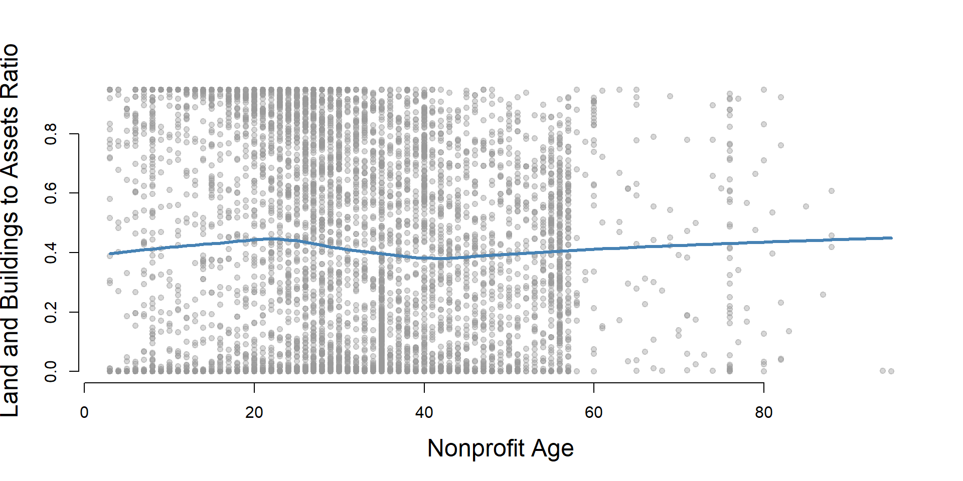
core2 %>%
  filter( ! is.na(age.q) ) %>%
  ggplot( aes(lb_to_assets) )  +
    geom_density( alpha = 0.5 ) +
    labs( title="Nonprofit Age" ) +
    xlab( variable.label ) +
    ylab( "" ) +
    facet_wrap( ~ age.q, nrow=3 ) +
    theme_minimal( base_size = 22 )  +
    theme( axis.title.y=element_blank(),
           axis.text.y=element_blank(),
           axis.ticks.y=element_blank() )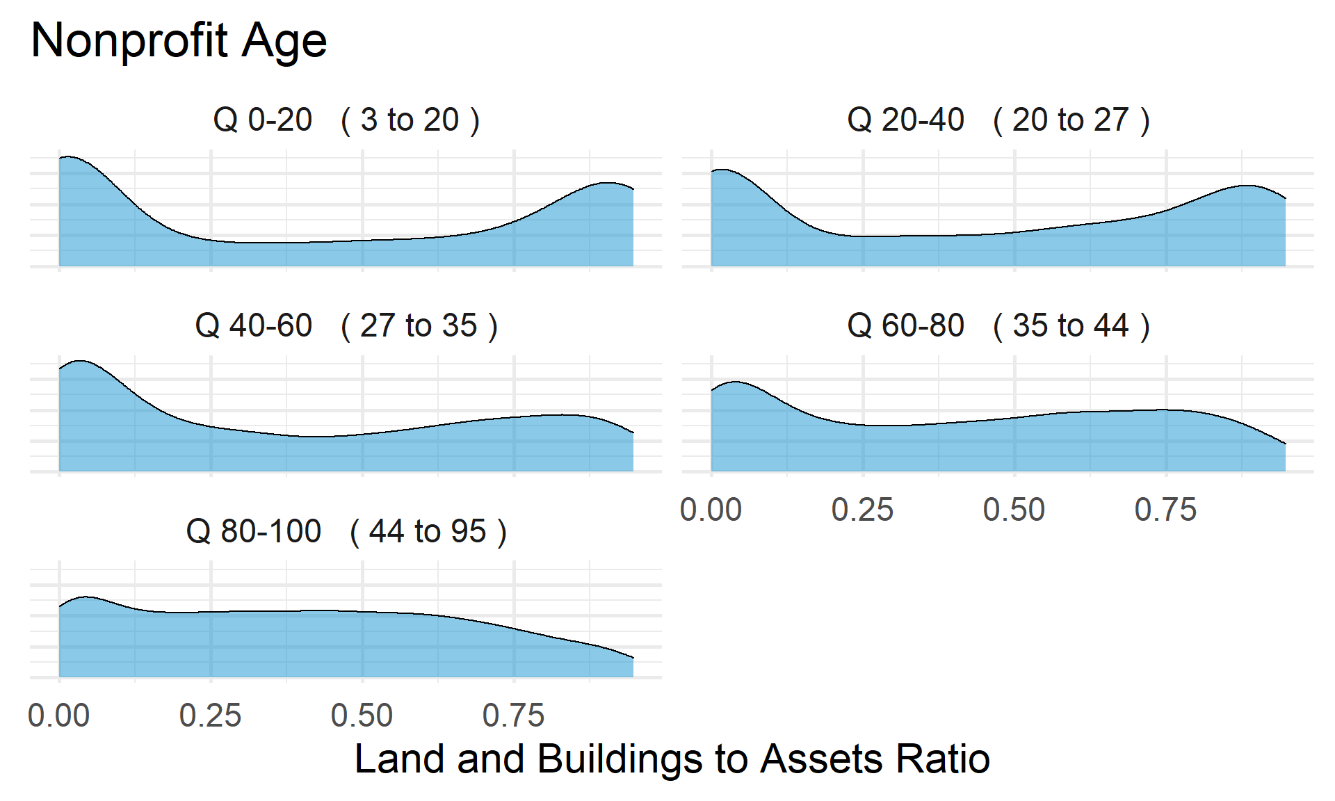
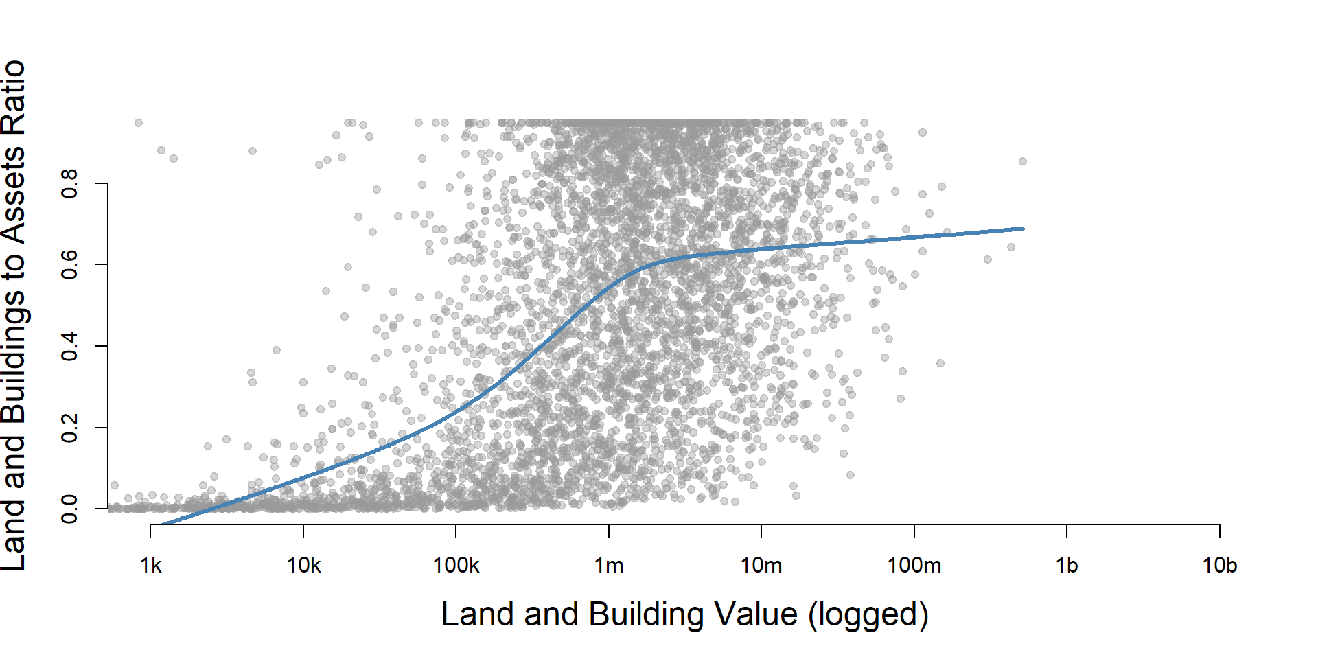
Land and Building Share by Land and Building Value
ggplot( core2, aes(x = lndbldgsequipend )) +
geom_density( alpha = 0.5 ) 
core2$lndbldgsequipend[ core2$lndbldgsequipend < 1 ] <- NA
if( nrow(core2) > 10000 )
{
  core3 <- sample_n( core2, 10000 )
} else
{
  core3 <- core2


jplot( log10(core3$lndbldgsequipend), core3$lb_to_assets,
       xlab="Land and Building Value (logged)",
       ylab=variable.label,
       xaxt="n", xlim=c(3,10) )
axis( side=1,
      at=c(3,4,5,6,7,8,9,10),
      labels=c("1k","10k","100k","1m","10m","100m","1b","10b") )
}
core2 %>%
  filter( ! is.na(land.q) ) %>%
  ggplot( aes(lb_to_assets) )  +
    geom_density( alpha = 0.5 ) +
    labs( title="Land and Building Value" ) +
    xlab( variable.label ) +
    ylab( "" ) +
    facet_wrap( ~ land.q, nrow=3 ) +
    theme_minimal( base_size = 22 )  +
    theme( axis.title.y=element_blank(),
           axis.text.y=element_blank(),
           axis.ticks.y=element_blank() )
Save Metrics
core.lb_to_assets <- select( core, ein, tax_pd, lb_to_assets )
saveRDS( core.lb_to_assets, "03-data-ratios/m-07-land-to-assets-ratio.rds" )
write.csv( core.lb_to_assets, "03-data-ratios/m-07-land-to-assets-ratio.csv" )